Topics in Computational Mechanics: Part 3

Recall the continuum approach to mechanics. We view the body, the structure of our interest, as a continuous region $\Omega$ in the vector space of $\mathbb{R}^{3}$. Then, we can completely describe the structure's state by finding the set of fields $\{\sigma,\,\varepsilon,\,\vec{u}\}$ that satisfies the force and moment equilibriums, the stress-strain relation (constitutive equation), and the strain-displacement relation (kinematics).

The problem is, finding the fields exactly is impossible for all but simple structures. Today, we will look at how to make the problem simpler so that we can analyze real-life structures.

1. Governing Equations: Elastostatics

If we assume small strain and linear elasticity, we can simplify the problem as follows: Find the stress field $\sigma = \sigma(\vec{x})$, the strain field $\varepsilon = \varepsilon(\vec{x})$, and the displacement field $\vec{u} = \vec{u}(\vec{x})$ that satisfy,

Equation 1.1. Elastostatics

$$\displaystyle\left.\begin{array}{l} -\text{div}(\sigma) = \vec{b},\,\,\,\,\,\sigma = \sigma^{T} \\ \sigma = C\varepsilon \\ \displaystyle\varepsilon = \frac{1}{2}\bigl(\nabla\vec{u} + \nabla\vec{u}^{T}\bigr) \end{array}\right/\,\,\,\begin{array}{l} -\sigma_{ij,j} = b_{i},\,\,\,\,\,\sigma_{ij} = \sigma_{ji} \\ \sigma_{ij} = C_{ijkl}\varepsilon_{kl} \\ \displaystyle\varepsilon_{ij} = \frac{1}{2}\bigl(u_{i,j} + u_{j,i}\bigr) \end{array},\,\,\,\forall\,\vec{x} \in \Omega$$

From top to bottom, we have the force and moment equilibriums, the stress-strain relation, and the strain-displacement relation. The left side shows how to write the equations using tensors, while the right side shows how to write at component level. Note that $\vec{b} = \vec{b}(\vec{x})$ is the body force, and $C = C(\vec{x})$ is a fourth-order elasticity tensor. We assume the standard basis that is aligned with the Cartesian coordinates.

The stress, strain, and displacement fields must also satisfy the displacement and traction conditions that are prescribed on the boundary $\partial\Omega$, i.e. the surface of the structure. Under minor assumptions, we can prove that the solution $\{\sigma,\,\varepsilon,\,\vec{u}\}$ to this boundary value problem exists and is unique.

Normally, a fourth-order tensor can have $3^{4} = 81$ independent components (each component is a function of the position vector $\vec{x}$). Because the elasticity tensor $C$ satisfies major and minor symmetries, it can only have 21 independent components. But twenty-one is still too many!

If we assume that the structure is made from an isotropic, homogeneous material, the elasticity tensor $C$ simply depends on two constants. Yep, you read that right. Just two components, both independent of the location $\vec{x}$. We can use Lamé's modulus $\lambda$ and the shear modulus $\mu$ to write,

Equation 1.2. Elasticity tensor for isotropic, homogeneous structure

$$\displaystyle\left.C = \lambda\,\bigl(I \otimes I\bigr) + 2\mu\,\mathbb{I}_{sym}\,\,\,\,\right/\,\,\,C_{ijkl} = \lambda\,\delta_{ij}\delta_{kl} + 2\mu \cdot \frac{1}{2}\bigl(\delta_{ik}\delta_{jl} + \delta_{il}\delta_{jk}\bigr)$$

Depending on the application, we can use Young's modulus $E$ and Poisson's ratio $\nu$ instead to more easily describe the problem and solution.

Lastly, let's combine the three equations in 1.1 and use the elasticity tensor in 1.2. Then, the equations that describe the structure's behavior solely depend of 3 displacement fields $u_{1} \equiv u$, $u_{2} \equiv v$, and $u_{3} \equiv w$:

Equation 1.3. Elastostatics for isotropic, homogeneous structure

$$\displaystyle -\mu\,u_{i,jj} - (\lambda + \mu)\,u_{j,ji} = b_{i},\,\,\,\forall\,\vec{x} \in \Omega$$

We have second-order partial differential equations (PDEs). This means a few omens. The displacements $u$, $v$, and $w$ must be twice-differentiable at all points in the body. At the same time, the 0th and 1st derivatives of displacements must match the prescribed displacements and tractions on the boundary. As if two omens aren't bad enough, the displacements are also coupled (we can't solve them one at a time), since they appear in all three equations.

In short, finding the exact solution to equation 1.3 is very difficult.

We know that the solution exists and is unique, however. Instead of the exact solution, we can find a numerical approximation. Depending on the geometry of the structure or the applied loads, we may even assume that the stresses, strains, or displacements will behave in a special way (e.g. they are numerically negligible, they don't depend on one of the coordinates, etc.) so that we can simplify the governing equations.

This is how we had arrived at the 1D, decoupled ordinary differential equations (ODEs) for trusses and beams. We used finite element method to approximately solve these equations. Once we found the approximations to displacements, we calculated the approximate strains and stresses using the strain-displacement relation and the stress-strain relation (equation 1.1).

2. Galerkin Method

The Galerkin method allows us to change a problem involving a continuous operator into a discrete problem. In simple terms, continuous means that the solution exists in an infinite-dimensional space (it's really hard to find!). Discrete means, the solution exists in a finite-dimensional subspace (easier to find). We call the original, difficult problem, the strong form, and the easier problem, the weak form.

We illustrate the Galerkin method for a truss-like or beam-like structure (a bar). The bar occupies the space $\Omega = (0,\,L) \times A$, where $L$ represents the length of the bar and $A = A(x)$, the cross-sectional area. For this bar problem, $x$, $y$, and $z$ denote the local coordinates that are aligned with the neutral axis ($x$) and the principal directions ($y$, $z$) of the area moment of inertia tensor. We use these coordinates to decouple the effects of stretching, bending, and twisting.

We will assume that the Young's modulus $E$, shear modulus $\mu$, cross-sectional area $A$, area moments of inertia $I_{y}$ and $I_{z}$, and polar moment of inertia $J$ are smooth functions of $x$, so that the strong and weak forms make sense. Oftentimes, for toy problems, we assume that these are all constant functions for simplicity.

For a truss-like bar, we allow an axial load $f = f(x)$ in the $x$ direction to cause the bar to axially displace by $u = u(x)$. For a beam-like bar, we allow a lateral load $g = g(x)$ in the $y$ direction, which causes the bar to laterally displace by $v = v(x)$ and rotate about the $z$ axis by $\theta_{z} \approx v' = v'(x)$.

If we are really ambitious, we can also study the effect of a lateral load $h = h(x)$ in the $z$ direction on the lateral displacement $w = w(x)$ and the rotation about the $y$ axis $\theta_{y} \approx -w' = -w'(x)$, as well as the effect of a twisting load $m = m(x)$ on the rotation about the $x$ axis $\theta_{x} = \theta_{x}(x)$.

Below, we neglect the effect of boundary conditions. It is important, however, to know that the type of BCs (i.e. Dirichlet, Neumann, or mixed) do influence which spaces we should look at for the solution and the test functions. For simplicity, we also neglect the body forces, and assume that no concentrated forces or concentrated moments are applied to the surface.

a. Strong form

For the truss and beam, the governing equations are as follows:

Equation 2.1. Truss

Find $u \in C^{2}(0,\,L)$ that solves,

$$\begin{array}{rl} \displaystyle-\frac{d}{dx}\Bigl(EA\,\frac{du}{dx}\Bigr) = f, & \forall\,x \in (0,\,L) \end{array}$$

Equation 2.2. Beam

Find $v \in C^{4}(0,\,L)$ that solves,

$$\begin{array}{rl} \displaystyle\frac{d^{2}}{dx^{2}}\,\Bigl(EI_{z}\,\frac{d^{2}v}{dx^{2}}\Bigr) = g, & \forall\,x \in (0,\,L) \end{array}$$

For a frame under the lateral load $h$ and the twisting load $m$, we must solve two more equations:

Equation 2.3. Frame

Find $w \in C^{4}(0,\,L)$ and $\theta_{x} \in C^{2}(0,\,L)$ that solve,

$$\begin{array}{rl} \displaystyle\frac{d^{2}}{dx^{2}}\,\Bigl(EI_{y}\,\frac{d^{2}w}{dx^{2}}\Bigr) = h, & \forall\,x \in (0,\,L) \\ \displaystyle-\frac{d}{dx}\Bigl(\mu J\,\frac{d\theta_{x}}{dx}\Bigr) = m, & \forall\,x \in (0,\,L) \end{array}$$

b. Weak form

Let me introduce the idea of weighted residual to create the weak form. Given some equation to solve, we can move everything to one side of the equation to define the residual function (error function).

For example, for the truss equation, the residual $r = r(x)$ is given by,

$$\displaystyle r \equiv -\frac{d}{dx}\Bigl(EA\,\frac{du}{dx}\Bigr) - f$$

We see that solving the equation is equivalent to requiring the residual function to be identically zero (the zero function).

Again, that requirement is too strong. We weaken it by testing whether the residual is zero "on average." What does average mean?

$$\displaystyle \int\limits_{0}^{L}\,r\varphi\,\,dx = 0,\,\,\,\forall\,\varphi \in H^{1}(0,\,L)$$

Let's break this down. We first multiplied the residual by a test function $\varphi$. The test function can be arbitrary, as long as it lives in the right test space (here, a Sobolev space called $H^{1}$). Then, we checked whether the integral of the product equals 0. Certainly, if the residual is zero, then the integral is zero. Conversely, if the integral is zero, then we can expect the residual to be almost zero.

Last but not least, we perform integration by parts (formally, i.e. we assume that the integration makes sense) to arrive at the weak form:

Equation 2.4. Truss

Find $u \in H^{1}(0,\,L)$ that solves,

$$\begin{array}{rl} \displaystyle\int\limits_{0}^{L}\,EA\,u'\varphi'\,\,dx = \int\limits_{0}^{L}\,f\varphi\,\,dx + \Bigl[EA\,u'\varphi\Bigr]_{0}^{L}, & \forall\,\varphi \in H^{1}(0,\,L) \end{array}$$

If there is a function $u$ that satisfies this equation for all test functions $\varphi$, then we can expect $u$ to be a good approximation to the exact solution.

Galerkin method is a special case of weighted residual method. For Galerkin method, we choose the test space (where $\varphi$ lives) to be the same as the solution space (where $u$ lives). We can expect nice mathematical results when the solution and test spaces are the same.

For brevity, let me just list the weak form for the beam equation. Because the beam equation has a fourth derivative, you would perform integration by parts twice.

Equation 2.5. Beam

Find $v \in H^{2}(0,\,L)$ that solves,

$$\begin{array}{rl} \displaystyle\int\limits_{0}^{L}\,EI_{z}\,v''\varphi''\,\,dx = \int\limits_{0}^{L}\,g\varphi\,\,dx - \left[\frac{d}{dx}\Bigl(EI_{z}\,v''\Bigr)\varphi - EI_{z}\,v''\varphi'\right]_{0}^{L}, & \forall\,\varphi \in H^{2}(0,\,L) \end{array}$$

c. Finite-dimensional subspace

The weak form is still hard to solve. The Sobolev spaces $H^{1}$ and $H^{2}$ have a dimension of infinity, so we can't search for the solution in practical time. We need to introduce a subspace $S$ with a finite dimension.

For the $H^{1}$ space, we can choose $S$ to be the space of piecewise linear polynomials. A function that lives in $S$ is guaranteed to be $C^{0}$-continuous, i.e. the function (its zeroth derivative) is continuous (there is no jump in the graph).

For brevity, let me omit details about creating a finite-dimensional basis of $S$ so that the resulting matrix $K$ will be sparse. For more information, please check the solutions to exercise problems.

Equation 2.6. Truss

Find $u \in S$ that solves,

$$\begin{array}{rl} \displaystyle\int\limits_{0}^{L}\,EA\,u'\varphi'\,\,dx = \int\limits_{0}^{L}\,f\varphi\,\,dx + \Bigl[EA\,u'\varphi\Bigr]_{0}^{L}, & \forall\,\varphi \in S \end{array}$$

For $H^{2}$, we can choose $S$ to be the space of piecewise cubic Hermite polynomials. A function that lives in $S$ is guaranteed to be $C^{1}$-continuous, i.e. the function and its first derivative are continuous.

Equation 2.7. Beam

Find $v \in S$ that solves,

$$\begin{array}{rl} \displaystyle\int\limits_{0}^{L}\,EI_{z}\,v''\varphi''\,\,dx = \int\limits_{0}^{L}\,g\varphi\,\,dx - \left[\frac{d}{dx}\Bigl(EI_{z}\,v''\Bigr)\varphi - EI_{z}\,v''\varphi'\right]_{0}^{L}, & \forall\,\varphi \in S \end{array}$$

d. Matrix equation

Once we assemble the element matrices and apply the BCs, we will end up with the matrix equation $K\vec{u} = \vec{f}$, where $K$ is a symmetric, positive definite (SPD) matrix. By choosing the right basis for $S$, the matrix $K$ can be sparse too, i.e. many of its entries will be zero. We have computationally efficient methods for solving the equation for sparse, SPD matrices, such as preconditioned conjugate gradient.

Equation 2.8. Truss and beam

Find $\vec{u} \in \mathbb{R}^{n}$ that solves,

$$\displaystyle K\vec{u} = \vec{f}$$

3. Energy Minimization Method

The Galerkin method may have come naturally to you if you are a mathematician and had experience with linear subspace and finite element method. If you are an engineer, you may prefer a physical explanation.

Here, we outline the Principle of Minimum Potential Energy for the truss and beam-like bars that we considered previously. The principle says that, among all displacements that satisfy the prescribed BCs, the displacement that satisfies the equilibrium equation is exactly the displacement with the least potential energy.

After defining the potential energy, we can use either calculus of variations or the Ritz method to find a numeric solution to the minimization problem. Again, for simplicity, we neglect boundary conditions, body force, and concentrated forces and moments on the surface.

a. Energy functional

We define the total potential energy $\Pi$ to be the sum of the internal strain energy and the external potential energy due to the applied loads. For dynamics, there would be an additional contribution from the kinetic energy.

Equation 3.1. Truss

Find $u \in C^{2}(0,\,L)$ that minimizes,

$$\displaystyle\Pi(u) = \frac{1}{2}\,\int\limits_{0}^{L}\,EA\,(u')^{2}\,\,dx - \int\limits_{0}^{L}\,fu\,\,dx$$

Equation 3.2. Beam

Find $v \in C^{4}(0,\,L)$ that minimizes,

$$\displaystyle\Pi(v) = \frac{1}{2}\,\int\limits_{0}^{L}\,EI_{z}\,(v'')^{2}\,\,dx - \int\limits_{0}^{L}\,gv\,\,dx$$

b. Calculus of variations

By taking the variational derivative (also called functional derivative) of $\Pi$, we get the differential equation that the minimizer must satisfy. This equation is called the Euler-Lagrange equation.

Below, we see that the Euler-Lagrange equations are exactly the governing equations (strong forms) for trusses and beams.

Equation 3.3. Truss

Find $u \in C^{2}(0,\,L)$ that solves,

$$\begin{array}{rl} \displaystyle-\frac{d}{dx}\Bigl(EA\,\frac{du}{dx}\Bigr) = f, & \forall\,x \in (0,\,L) \end{array}$$

Equation 3.4. Beam

Find $v \in C^{4}(0,\,L)$ that solves,

$$\begin{array}{rl} \displaystyle\frac{d^{2}}{dx^{2}}\,\Bigl(EI_{z}\,\frac{d^{2}v}{dx^{2}}\Bigr) = g, & \forall\,x \in (0,\,L) \end{array}$$

Just like before, we find the weak forms and introduce a finite-dimensional subspace.

c. Ritz method

Calculus of variations means, we take the variational derivative first, then introduce a finite-dimensional subspace. In Ritz method, we reverse the order. We introduce a finite-dimensional subspace first, then take the derivative (the gradient) to find the minimum. Often, the two approaches will yield the same discrete problem.

To illustrate, we look at minimizing the energy within a finite-dimensional subspace. For trusses, the minimizer lives in the space of piecewise linear polynomials. For beams, in the space of piecewise cubic Hermite polynomials.

Equation 3.5. Truss

Find $u_{h} \in S$ that minimizes,

$$\displaystyle\Pi(u_{h}) = \frac{1}{2}\,\int\limits_{0}^{L}\,EA\,(u_{h}')^{2}\,\,dx - \int\limits_{0}^{L}\,fu_{h}\,\,dx$$

Equation 3.6. Beam

Find $v_{h} \in S$ that minimizes,

$$\displaystyle\Pi(v_{h}) = \frac{1}{2}\,\int\limits_{0}^{L}\,EI_{z}\,(v_{h}'')^{2}\,\,dx - \int\limits_{0}^{L}\,gv_{h}\,\,dx$$

The minimizer must satisfy the discrete equation $\nabla\Pi = \vec{0}$ (this is the weak form).

d. Matrix equation

Equation 3.7. Truss and beam

Find $\vec{u} \in \mathbb{R}^{n}$ that solves,

$$\displaystyle K\vec{u} = \vec{f}$$

e. Proof of Principle of Minimum Potential Energy

Recall that, among all displacements that satisfy the prescribed BCs, the displacement that satisfies the equilibrium equation is the same as the displacement with the least potential energy.

The statement "if the potential energy is minimum, then the minimizing displacement satisfies the equilibrium equation" comes from calculus of variations.

Here, we prove the converse statement "if the displacement satisfies the equilibrium equation, then the potential energy is at minimum" for trusses. As an illustration, we consider the BCs $u(0) = u_{0}$ and $u(L) = u_{L}$.

By assumption, the displacement field $u = u(x)$ satisfies the equilibrium equation,

$$\begin{array}{rl} \displaystyle-\frac{d}{dx}\Bigl(EA\,\frac{du}{dx}\Bigr) = f, & \forall\,x \in (0,\,L)\end{array}$$

The potential energy due to this displacement is,

$$\displaystyle\Pi(u) = \frac{1}{2}\,\int\limits_{0}^{L}\,EA\,(u')^{2}\,\,dx - \int\limits_{0}^{L}\,fu\,\,dx$$

Consider another displacement $w$ that also satisfies the BCs $w(0) = u_{0}$, $w(L) = u_{L}$, but is a function different from $u$. We can then write $w = u + v$ for some function $v \neq 0$. The field $v$ satisfies the homogeneous BCs $v(0) = 0$ and $v(L) = 0$.

The potential energy due to the displacement field $w$ is,

$$\begin{array}{l} \begin{aligned} \Pi(w) &= \frac{1}{2}\,\int\limits_{0}^{L}\,EA\,(u' + v')^{2}\,\,dx - \int\limits_{0}^{L}\,f(u + v)\,\,dx \\ &= \frac{1}{2}\,\int\limits_{0}^{L}\,EA\,(u')^{2}\,\,dx + \int\limits_{0}^{L}\,EA\,u'v'\,\,dx + \frac{1}{2}\,\int\limits_{0}^{L}\,EA\,(v')^{2}\,\,dx - \int\limits_{0}^{L}\,fu\,\,dx - \int\limits_{0}^{L}\,fv\,\,dx \\ &= \Pi(u) \,+\, \underbrace{\int\limits_{0}^{L}\,EA\,u'v'\,\,dx \,- \int\limits_{0}^{L}\,fv\,\,dx}_{\text{linear term in v}} \,+ \underbrace{\frac{1}{2}\,\int\limits_{0}^{L}\,EA\,(v')^{2}\,\,dx}_{\small\text{quadratic term in v}} \end{aligned} \end{array}$$

Because the function $v$ is not identically zero, we have $v'(x) \neq 0$ at some region of $(0,\,L)$. Hence, the quadratic term is some positive number.

As for the linear term in $v$, we integrate by parts to get,

$$\displaystyle\text{linear term in v} \,=\, \underbrace{\int\limits_{0}^{L}\,\left(-\frac{d}{dx}\Bigl(EA\,\frac{du}{dx}\Bigr) - f\right)v\,\,dx}_{=\,0} + \underbrace{\Bigl[EA\,u'v\Bigr]_{0}^{L}}_{=\,0} \,=\, 0$$

This is because $u$ satisfies the equilibrium equation over $(0,\,L)$, while $v$ satisfies the BCs $v(0) = v(L) = 0$.

Therefore, we conclude that the potential energy due to the equilibrium displacement $u$ is at minimum:

$$\begin{array}{rl} \displaystyle\Pi(w) > \Pi(u), & \forall\,w \neq u \end{array}$$

4. Exercises

Until now, our approach to solving elasticity problems has been heavy with theory. Let's better understand how to solve them with examples. I encourage you to follow along my solutions and see how the theory comes into play.

a. Problem 1

Recall the 5-bar truss problem from Part 1.

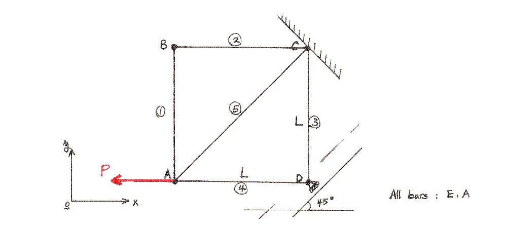
We showed that, after we apply the displacement BCs $u_{C,x} = 0$, $u_{C,y} = 0$, and $u_{D,y} = u_{D,x}$, the stiffness matrix equation reduces to,

$$\displaystyle\frac{EA}{L}\left[\begin{array}{cc|cc|c} \displaystyle 1 + \frac{1}{2\sqrt{2}} & \displaystyle\frac{1}{2\sqrt{2}} & & & -1 \\ \displaystyle\frac{1}{2\sqrt{2}} & \displaystyle 1 + \frac{1}{2\sqrt{2}} & & -1 & \\ \hline & & 1 & & \\ & -1 & & 1 & \\ \hline -1 & & & & 2 \end{array}\right] \left[\begin{array}{c} u_{A,x} \\ u_{A,y} \\ u_{B,x} \\ u_{B,y} \\ u_{D,x} \end{array}\right] = \left[\begin{array}{c} -P \\ 0 \\ 0 \\ 0 \\ 0 \end{array}\right]$$

Obtain this equation again by, instead, minimizing the potential energy of the system. Use linear polynomials to approximate the axial displacement of each bar.

b. Problem 2

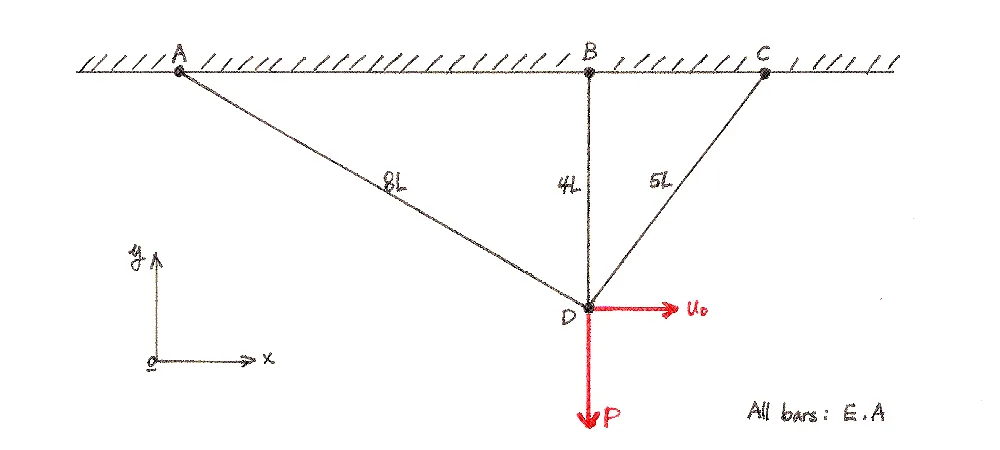
Consider the following truss. Find the $y$-displacement of node D by minimizing the potential energy of the system (use linear polynomials).

c. Problem 3

Consider a bar that is fixed to a wall on one end, while subjected to a compressive load $P$ on the other. There is also an internal axial load $f = f(x)$ (per unit length) that makes the bar want to stretch. We are interested in how the bar deforms axially due to these two loads.

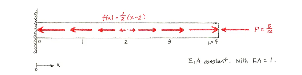
(a) Write down the governing equation for the axial displacement $u = u(x)$ and the BCs that it satisfies. Solve this equation to find that,

$$\displaystyle u(x) = -\frac{1}{12}\,x^{3} + \frac{1}{2}\,x^{2} - \frac{5}{12}\,x,\,\,\,\forall\,x \in [0,\,4]$$

(b) State the weak form of the governing equation. Then, introduce a finite-dimensional subspace $S$ of piecewise linear polynomials, using 1, 2, and 4 elements of equal size. (That's three subspaces to consider!)

(c) Find the FE solution $u_{h} \in S$ to the weak form, for the cases of 1, 2, and 4 elements. How does the graph of the FE solution $u_{h}$ compare to that of the exact solution $u$, in particular, as we increase the number of elements from 1 to 2 to 4?

(We can more objectively measure the error using energy, $L^{2}$, or $L^{\infty}$ norm.)

d. Problem 4

For each strong form, identify (or draw) the physical problem and state the weak form. (Finding the correct solution and test spaces is optional.) Assume that the distributed loads and material parameters are sufficiently smooth functions and allow integration by parts to make sense.

(a) Find $u \in C^{2}(0,\,L)$ such that,

$$\left\{\begin{array}{l} \displaystyle -\frac{d}{dx}\Bigl(EA\,\frac{du}{dx}\Bigr) = \cos\Bigl(\frac{x}{L}\,\pi\Bigr),\,\,\,\forall\,x \in (0,\,L) \\ u(0) = 0,\,\,\,u(L) = 0 \end{array}\right.$$

(b) Find $u \in C^{2}(0,\,L)$ such that,

$$\left\{\begin{array}{l} \displaystyle -\frac{d}{dx}\Bigl(EA\,\frac{du}{dx}\Bigr) = 0,\,\,\,\forall\,x \in (0,\,L) \\ (EA\,u')(0) = -1,\,\,\,u(L) = 2 \end{array}\right.$$

(c) Find $v \in C^{4}(0,\,L)$ such that,

$$\left\{\begin{array}{l} \displaystyle \frac{d^{2}}{dx^{2}}\Bigl(EI_{z}\,\frac{d^{2}v}{dx^{2}}\Bigr) = -1,\,\,\,\forall\,x \in (0,\,L) \\ v(0) = 0,\,\,\,v'(0) = 0,\,\,\,v(L) = 0,\,\,\,(EI_{z}\,v'')(L) = 1 \end{array}\right.$$