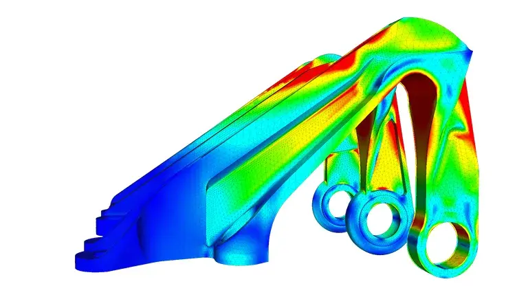
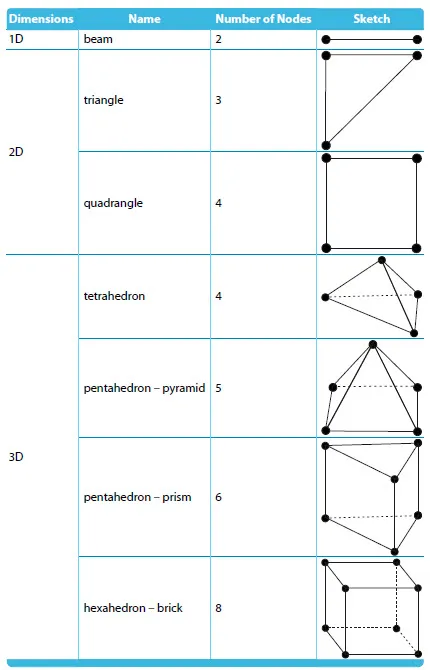
The geometries that we considered so far are simple. If we are to analyze a complex, real-world structure, we need a way to accurately model its geometry. Not to worry, we can map a simple element to a complex one using a function.
Today, we will study the isoparametric approach. It tells us how to define the function so that we can evaluate integrals fast and achieve optimal rate of convergence. It is key to making FEM practical and powerful.
1. Isoparametric Approach
We begin with an element in the parametric space. The parametric space is named so because the element gets to take a simple shape—one that we can easily define with parameters. For example, we use a line segment in 1D, a triangle or square in 2D, and a tetrahedron or cube in 3D. The element also provides nodes—special points that let us define a basis of functions. Because we will use this element to create other elements, we refer to it as the parent domain.
Once we have such element in the parametric space, we can create a function to map that element into the physical space. The physical space is where the structure of our interest lives. Because we mapped (transformed) the element, the element can take a complex shape in the physical space.
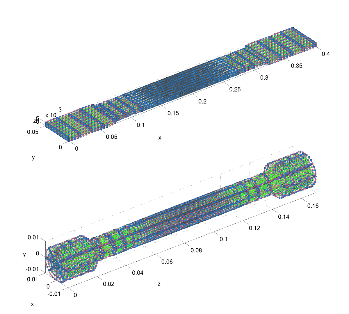
Thanks to the idea of parametric and physical spaces, we can build complicated geometries easily. Both rectangular and circular bars above came from the same "stack of boxes" in the parametric space.
For our study, we assume that the function is bijective, i.e. the inverse function exists. The inverse allows us to map the complex element (in the physical space) back to the simple element (in the parametric space). This ability becomes crucial for integrations. Note that, for certain problems, the inverse may not exist everywhere, or may collapse into a singularity. Dealing with numerical instability is topic for another day.
There is more than one way to map the parametric space to the physical space. This is where isoparametric approach comes in. It tells us to use the same basis functions to achieve two goals: (1) map the parent domain to an element in the physical space, i.e. describe the geometry; and (2) define the FE solution inside the element, i.e. describe the field that we are interested in.
Furthermore, an isoparametric approach ensures convergence. As we use more and more elements to describe the geometry (i.e. decrease the element size), we expect the FE solution to converge to the exact solution, point-wise (strong sense) or in some weak sense. The sufficient conditions for convergence are to use the right basis—one that meets the level of smoothness required by the weak form, and forms a partition of unity—and to follow the isoparametric approach.
Since 2005, the isogeometric approach (IGA) has been pursued by both academic and engineering communities. Here, B-splines, NURBS, and T-splines, which are readily available in CAD (computer-aided design), serve as basis for the geometry and fields. To highlight the fact that the geometry is represented exactly with B-splines, NURBS, and T-splines—versus approximately with polynomials—we call this isoparametric approach, isogeometric. IGA gives us competitive, if not better, results over the usual isoparametric approaches.
Next, we take a look at how to apply isoparametric approach to solve 1D elastostatics problems. We consider two types of 1D elements for a compare-and-contrast.
a. Two-noded, linear elements (1D)
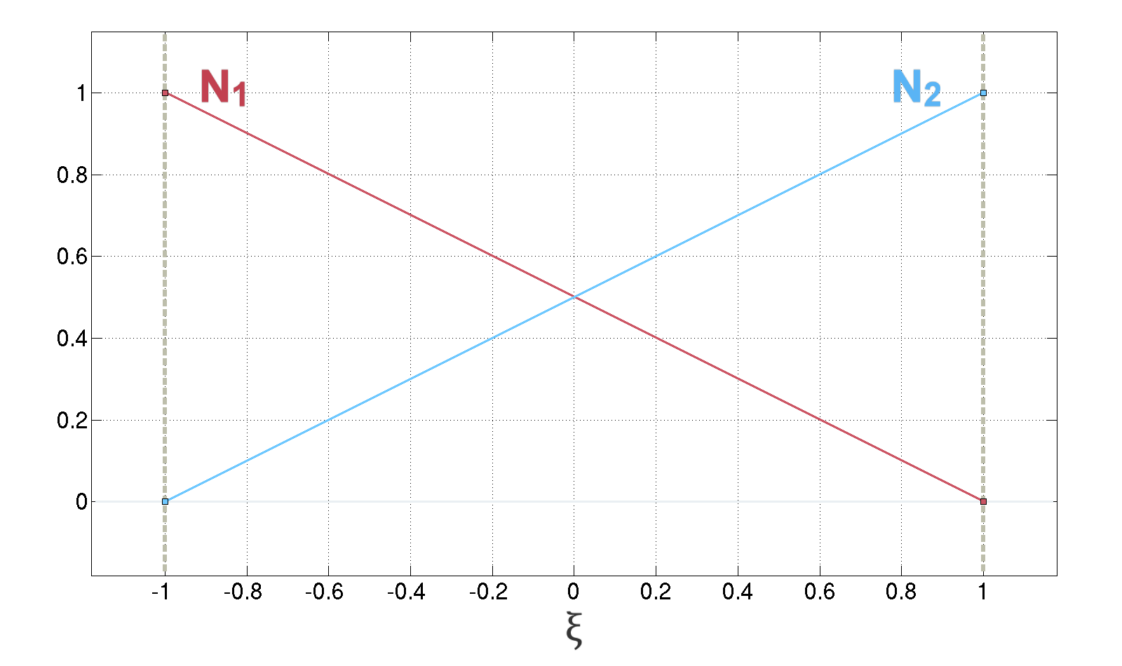
Consider two linear functions N1=N1(ξ) and N2=N2(ξ), which are defined over the parent domain, the closed interval [−1,1].
Equation 1.1. Basis functions for the parent domain
N1(ξ)=−21ξ+21N2(ξ)=21ξ+21
These functions are interpolatory. It means, we satisfy the equation Ni(ξj)=δij at the nodes ξ1=−1 and ξ2=1. We can also check that N1 and N2 form a basis for the set of linear polynomials over the parent domain, i.e. any linear function over [−1,1] can be written as a linear combination of N1 and N2.
Linear basis functions for the parent domain.
We need to create a linear function x=x(ξ) that can map the parent domain [−1,1] to any two-noded element e=[x1,x2] in the physical space. Because the basis functions N1 and N2 are interpolatory, we deduce that the map is,
Note that the derivative of the map is a constant function,
dξdx(ξ)=2x2−x1
and, more importantly, that the derivative is positive for all ξ \in (−1,1).
Inverse Function Theorem (1D)
Let x=x(ξ) be a map from [a,b] to [c,d]. If the map is Ck(a,b) for some k≥1 and its JacobianJ(ξ)≡(dx/dξ)(ξ) is positive for all ξ∈(a,b), then the inverse map ξ=ξ(x) exists and is Ck(c,d).
We can generalize this result to higher dimensions. The Jacobian is defined as the determinant of the Jacobian matrix.
Since the derivative is positive, the Inverse Function Theorem tells us that the inverse map ξ=ξ(x) exists, i.e. we can always return to the parent domain from any element in the physical space. We need this ability to calculate integrals fast and accurately. In general, we can't write an explicit formula for the inverse map. Luckily, its existence is enough for us.
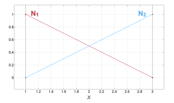
To follow the isoparametric approach, we define the basis functions N1(x) and N2(x) for the physical element to be the composite functions N1(ξ(x)) and N2(ξ(x)).
Equation 1.2. Basis functions for the element
N1(x)≡N1(ξ(x))N2(x)≡N2(ξ(x))
Notice the abuse of notation. The N1 and N2 on the left-hand side refer to the basis for the element in the physical space, whereas those on the right refer to the linear basis for the parent domain. I didn't use a different symbol for the physical basis because, from the context, it will always be clear which basis we are looking at.
Basis functions for an element in the physical space. This element has nodes at $$x_{1} = 1$$ and $$x_{2} = 3$$.
Lastly, we express the field of our interest in terms of the physical basis N1(x) and N2(x). In elastostatics, we want to know the displacement field u=u(x). Over the element e=[x1,x2], we define the FE solution uh to be,
uh(x)=u1N1(x)+u2N2(x)
for some coefficients u1 and u2.
Equation 1.3. Displacement field
uh(x)=u1N1(x)+u2N2(x)
Please note that, by N1(x) and N2(x) in equation 1.3, we do not mean "construct linear, interpolatory basis functions for the physical element, just like we did for the parent domain." What we really mean is, "find the value of ξ in the parent domain that will map to x, then evaluate N1(ξ) and N2(ξ)."
This distinction is hard to see for a linear basis, since the composite functions N1(ξ(x)) and N2(ξ(x)) happen to be linear polynomials in x. We will see with a quadratic basis that, in general, the basis functions for the physical element are not polynomials in x.
The element stiffness matrix Ke and the element load vector fe have integrals that are defined in the physical space. To evaluate them, we "pull back" to the parent domain and evaluate the integrals there. We can do this because the inverse map exists.
Recall that, for a truss-like bar under an axial load f=f(x), the entries of Ke and fe are given by,
Note that the quantities x1, x2, E(x), A(x), and f(x) are data that we need to provide in an input file. A mesh generator may also have the final say on where the nodes x1 and x2 should be placed.
b. Three-noded, quadratic elements (1D)
Consider three quadratic functions N1=N1(ξ), N2=N2(ξ), and N3=N3(ξ) over the parent domain [−1,1]:
Equation 1.5. Basis functions for the parent domain
N1(ξ)=21ξ2−21ξN2(ξ)=−ξ2+1N3(ξ)=21ξ2+21ξ
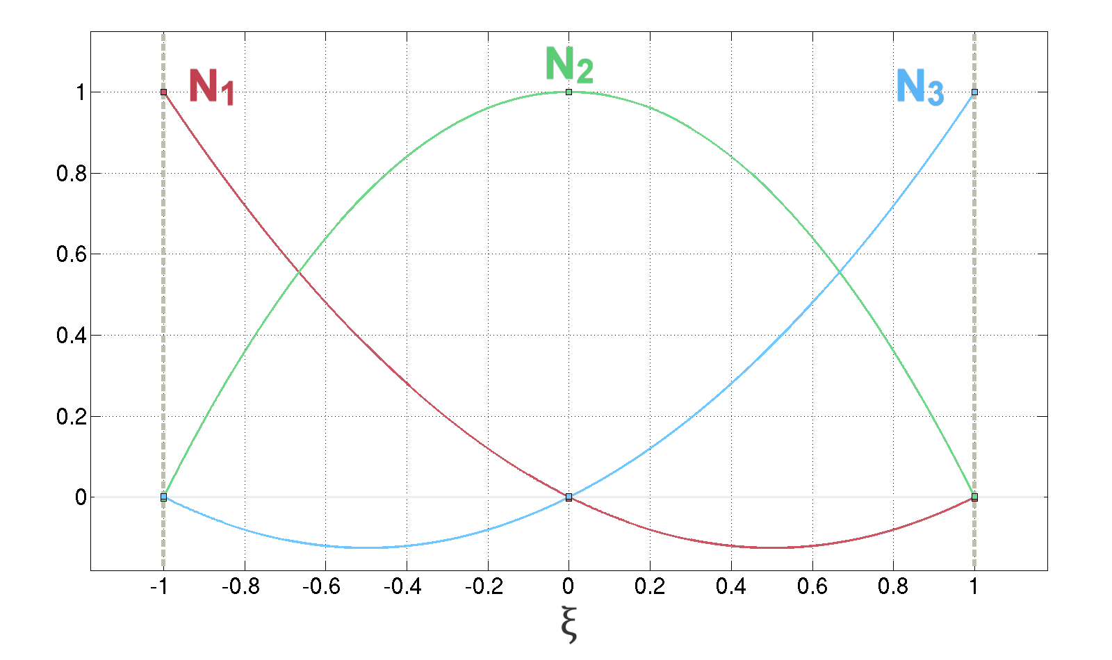
These functions satisfy the interpolatory property Ni(ξj)=δij for the nodes ξ1=−1, ξ2=0, and ξ3=1. They also form a basis for the quadratic polynomials over [−1,1].
Quadratic basis functions for the parent domain.
We now use N1, N2, and N3 to quadratically map the parent domain to a three-noded element e=[x1,x3] in the physical space (x2 is the node in-between):
x(ξ)=x1N1(ξ)+x2N2(ξ)+x3N3(ξ)
The derivative of the map is a linear function,
dξdx(ξ)=x1(ξ−21)+x2(−2ξ)+x3(ξ+21)
In order to use the Inverse Function Theorem, we must guarantee that the derivative (Jacobian) is positive for all ξ∈(−1,1).
We claim that, in order for the Jacobian J(ξ)=(dx/dξ)(ξ) to be positive for all ξ, the middle node x2 must be placed within a quarter distance from the element's center, (x1+x3)/2. In other words, if he≡x3−x1 denotes the size of the element, we must have,
x2∈(2x1+x3−4he,2x1+x3+4he)
To prove this, we only need to consider the case of x1=0 and x3=1. Stretching the element multiplies the Jacobian by some positive number, and translating it does not change the Jacobian.
Then,
J(ξ)=0⋅(ξ−21)+x2(−2ξ)+1⋅(ξ+21)=(1−2x2)ξ+21
We already see that, if x2=0.5 (we place the middle node at the element's center), then the Jacobian will be positive for all ξ∈(−1,1). What if we wanted to put the middle node somewhere else?
Well, consider the case of x2<0.5, which means the quantity (1−2x2) is positive. The fact that −1<ξ<1 implies the following inequality:
−(1−2x2)+21<J(ξ)<(1−2x2)+21
Since the Jacobian is positive for all ξ, if and only if, the lower bound of J(ξ) is positive, we must have,
x2>0.25
Finally, consider the case of x2>0.5, which means the quantity (1−2x2) is negative. The bound −1<ξ<1 implies,
−(1−2x2)+21>J(ξ)>(1−2x2)+21
Set the lower bound of J(ξ) to be greater than zero to conclude that,
x2<0.75
We define the basis functions N1(x), N2(x), and N3(x) for the physical element to be the composite functions N1(ξ(x)), N2(ξ(x)), and N3(ξ(x)).
Equation 1.6. Basis functions for the element
N1(x)≡N1(ξ(x))N2(x)≡N2(ξ(x))N3(x)≡N3(ξ(x))
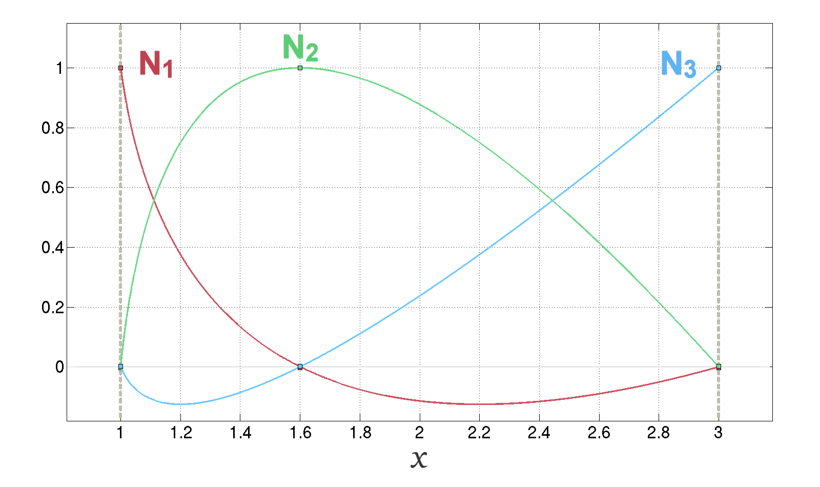
Basis functions for an element in the physical space. This element has nodes at $$x_{1} = 1$$, $$x_{2} = 1.6$$, and $$x_{3} = 3$$.
Lastly, we define the FE solution uh over the element e=[x1,x3] using these basis functions. In other words,
uh(x)=u1N1(x)+u2N2(x)+u3N3(x)
for some coefficients u1, u2, and u3.
Equation 1.7. Displacement field
uh(x)=u1N1(x)+u2N2(x)+u3N3(x)
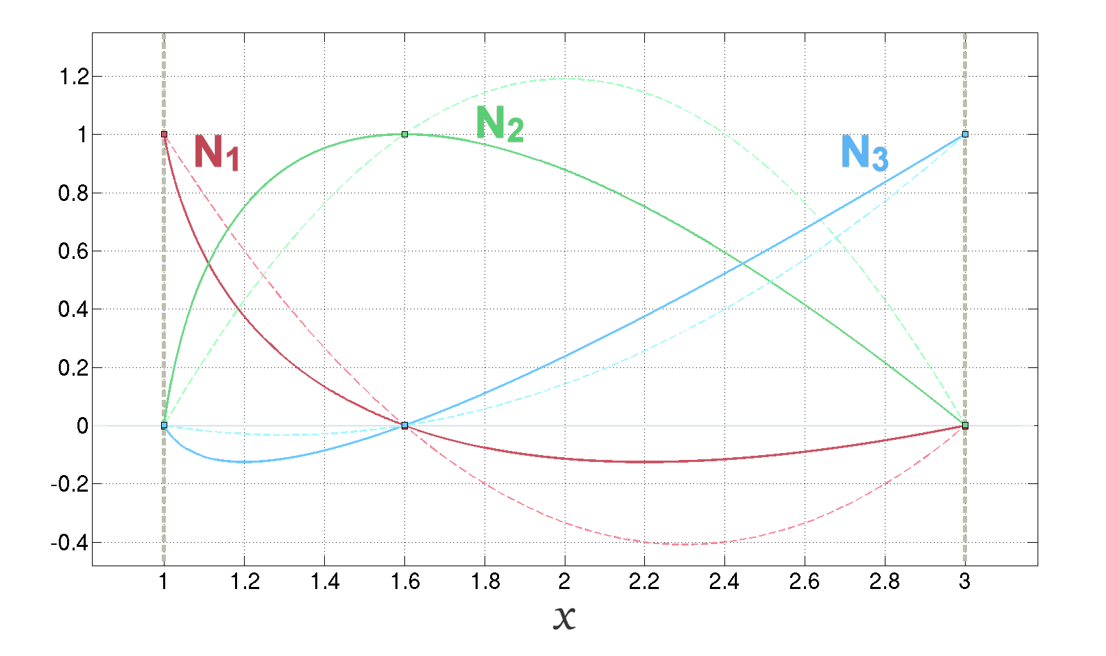
Again, by N1(x), N2(x), and N3(x) in equation 1.7, we don't mean "construct quadratic, interpolatory basis functions for the physical element." We really mean "find the value of ξ in the parent domain that will map to x, then evaluate N1(ξ), N2(ξ), and N3(ξ)." To make this distinction clear, the next figure shows what would happen we did construct quadratic, interpolatory basis functions on the physical space.
The quadratic, interpolatory basis functions on the physical space, which are shown in dashed lines, differ from the composite functions, shown in solid lines.
In general, the basis functions are not quadratic polynomials in x, because they are a composite function of a quadratic polynomial in ξ and the inverse map ξ(x), which takes on a complicated form. The only time that they are quadratic in x—the only time when we may make the mistake to create interpolatory functions in the physical space—is when the middle node x2=(x1+x3)/2 is placed at the element's center, just like how the node ξ2=0 was placed at the center of the parent domain. But this approach would severely limit the extent to which we can model the geometry.
For the truss problem, here are the entries of Ke and fe:
Again, we must provide the quantities x1, x2, x3, E(x), A(x), and f(x) in an input file. We must also place the node x2 within a quarter distance from the element's center.
2. Numerical Integration
In Section 1, we showed that the element stiffness matrices and element load vectors are computed in the parent domain [−1,1]. All that remains is to evaluate the integrals in equations 1.4 or 1.8. Clearly, there is no integration formula that will work for all user-defined functions E(x), A(x), and f(x). We turn to numerical integration, also known as quadrature.
Given a continuous function f=f(x) that is defined over the interval [−1,1], we want to approximate the integral
−1∫1f(x)dx
First, we sample the function at quadrature points x1,x2,⋯,xq∈[−1,1]. Evaluating the function is easy. Then, we can weigh the values by some numbers w1,w2,⋯,wq. Lastly, we combine the weighted values (i.e. take a linear combination) to approximate the integral:
−1∫1f(x)dx=w1f(x1)+w2f(x2)+⋯+wqf(xq)+error
Let's now take a look at how to choose the quadrature points and the weights so that we are guaranteed to have a good approximation (have a small error).
a. Newton-Cotes quadrature
The idea behind Newton-Cotes quadrature is simple: if we can approximate f with a polynomial p of degree (q−1), we can integrate the polynomial instead. Integrating a polynomial is easy.
We use the polynomial that interpolates f at the quadrature points, which are spaced evenly apart inside the domain (−1,1). We intentionally don't place quadrature points at the endpoints x=−1 and x=1, because the derivatives of the basis functions may be undefined at the element interfaces.
Therefore, let's look for the polynomial p that satisfies the equations,
p(x1)=f(x1)p(x2)=f(x2)⋮p(xq)=f(xq)
Such a polynomial exists and is unique because we can create Lagrange interpolation basis functions N1,N2,⋯,Nq (just like we did for the isoparametric approach):
In summary, for Newton-Cotes quadrature, where we sample is evenly spaced apart in the open domain (−1,1). How much weight we assign each sample is determined by the integral of the corresponding Lagrange interpolation basis function.
The table below shows the quadrature scheme for q=1,2,3,4.
If we use q quadrature points, the Newton-Cotes quadrature is exact for all functions that are polynomials of degree (q−1) or less. We can see this from the error term. xˉ represents some number in [−1,1] and differs from one quadrature to another.
The error also shows that, when q is odd, we get an extra accuracy. For example, the 3-point quadrature is exact for cubic polynomials, not just for quadratic polynomials. The 4-point quadrature is as accurate as the 3-point (it may have a smaller error), but requires us to evaluate f at one additional point.
b. Gauss quadrature
We arrived at a q-point quadrature that is exact for polynomials of degree (q−1) by assuming that the points are equally spaced apart.
If we instead optimize the locations of the quadrature points along with their weights, we get a quadrature that is optimal in 1D. Known as Gauss quadrature, it is exact for polynomials of degree up to (2q−1). Each additional quadrature point lets us double the degree of the polynomial that we can handle! No other q-point quadrature can achieve more accuracy in 1D.
Gauss quadrature comes from orthogonal polynomials called Legendre polynomials. The topic is out of scope, so I'll just list the quadrature scheme below:
We want to find the displacement field u∈R3 that satisfies the equation,
Ω∫σ:δεdV=Ω∫b⋅δudV+∂Ω∫t⋅δudS
for all admissible test functions δu∈R3. In the context of Principle of Virtual Work, we call test functions, virtual displacements.
Because the stress and strain tensors are symmetric, we can write their inner product σ:δε as the dot product between the stress "vector" and the (virtual) strain "vector" using the engineering strains. In other words,
We assume that this relation also holds for the virtual fields.
d. Finite-dimensional subspace
Finally, we approximate the displacement field and the virtual displacement field by following the isoparametric approach. For example, when we use tetrahedral linear elements, we have the following relation on each element:
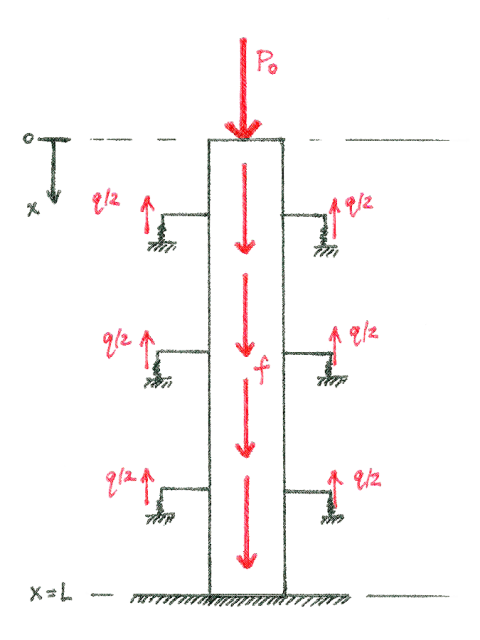
Consider a steel pile of length L=4m, Young's modulus E=210GPa, and cross-sectional area A=π(0.2)2m2.
A steel pile embedded in soil.
The pile is fixed at the bottom and is assumed to be a Winkler foundation across the length. In other words, we assume that the soil exerts a force that is opposite and linearly proportional to the displacement of the pile, i.e. q=q(x)=ku(x) for some constant k (called foundation stiffness). Note, q has the unit of N/m.
We want to know how the pile deforms due to the load P0=105N at its head, the distributed load f=f(x)N/m, and the lateral force q=ku(x) due to the soil. For simplicity, we consider k=EA/L2 and f(x)=P0/L below.
(a) From equilibrium of a differential element, derive the governing equation and the BCs for the displacement of the pile u=u(x).
(b) Find the weak form. Assuming an element has (p+1) basis functions, write down the element stiffness matrix and the element load vector.
(c) From the weak form, obtain the governing equation and the BCs that u satisfies. (In other words, show that we can return to the strong form.)
(d) Consider 1 element with a linear basis (p=1). Find the FE solution uh and calculate the internal force Fh(0)=EAuh′(0) at the pile head. What do you see?
(e) Now, consider 2 elements, each with a linear basis (p=1).
(f) Lastly, consider 1 and 2 elements with a quadratic basis (p=2) in each. Assume that the middle node is placed at the element's center.