In continuum mechanics, we view the body—the structure (solid or fluid) that is of our interest—as a continuous region that lives in the three-dimensional space $\mathbb{R}^{3}$ .

The word continuous means, we assume the body to be made up of infinitely many, infinitely small points, with no space in-between (like the cloud of paint seen above), rather than discrete, finitely small atoms, with an atomistic space in-between.

The space $\mathbb{R}^{3}$ is special in many ways (mathematically, that is), and allows us to set up and solve problems in mechanics in a rigorous manner. To keep things interesting and concise, we will replace some definitions with layman, more intuitive explanations.

1. Vector Space

a. $\mathbb{R}^{3}$ is a vector space

The elements in a vector space are called vectors. Addition and scalar multiplication of vectors are closed (we always stay inside the space) and follow certain axioms (rules). In other words, we can safely compute addition and scalar multiplication of vectors because they are well-defined operations.

A vector space always contains the zero vector $\vec{0}$ . We can arbitrarily assign a point in our physical world to be the origin. This allows us to identify points that make up the body as vectors in $\mathbb{R}^{3}$ (called position vectors in continuum mechanics).

b. $\mathbb{R}^{3}$ has a dimension of 3

We can find three vectors $\vec{e}_{1},\,\vec{e}_{2},\,\vec{e}_{3} \in \mathbb{R}^{3}$ that are linearly independent (quite literally, independent from one another) and span (cover) the entire space of $\mathbb{R}^{3}$ . The set of such vectors is called a basis and these vectors are called basis vectors.

Using basis vectors, we can write any vector $\vec{x} \in \mathbb{R}^{3}$ as their linear combination, i.e. there always exist scalars $x_{1},\,x_{2},\,x_{3} \in \mathbb{R}$ such that

$\displaystyle\vec{x} = x_{1}\vec{e}_{1} + x_{2}\vec{e}_{2} + x_{3}\vec{e}_{3}$

The representation of $\vec{x}$ in terms of the basis $\{\vec{e}_{1},\,\vec{e}_{2},\,\vec{e}_{3}\}$ is unique. There is no other set of scalars $\{x_{1}',\,x_{2}',\,x_{3}'\}$ such that $x_{1}'\vec{e}_{1} + x_{2}'\vec{e}_{2} + x_{3}'\vec{e}_{3}$ will also give us back $\vec{x}$ .

What does this mean? As long as we have 3 vectors that form a basis, we can locate any point in the body and describe mathematically what is happening physically at a point and its nearby points. For example, we can talk about a point in terms of its x, y, and z coordinates (Cartesian coordinates). We can also talk about it in terms of radius, latitude, and longitude (spherical coordinates).

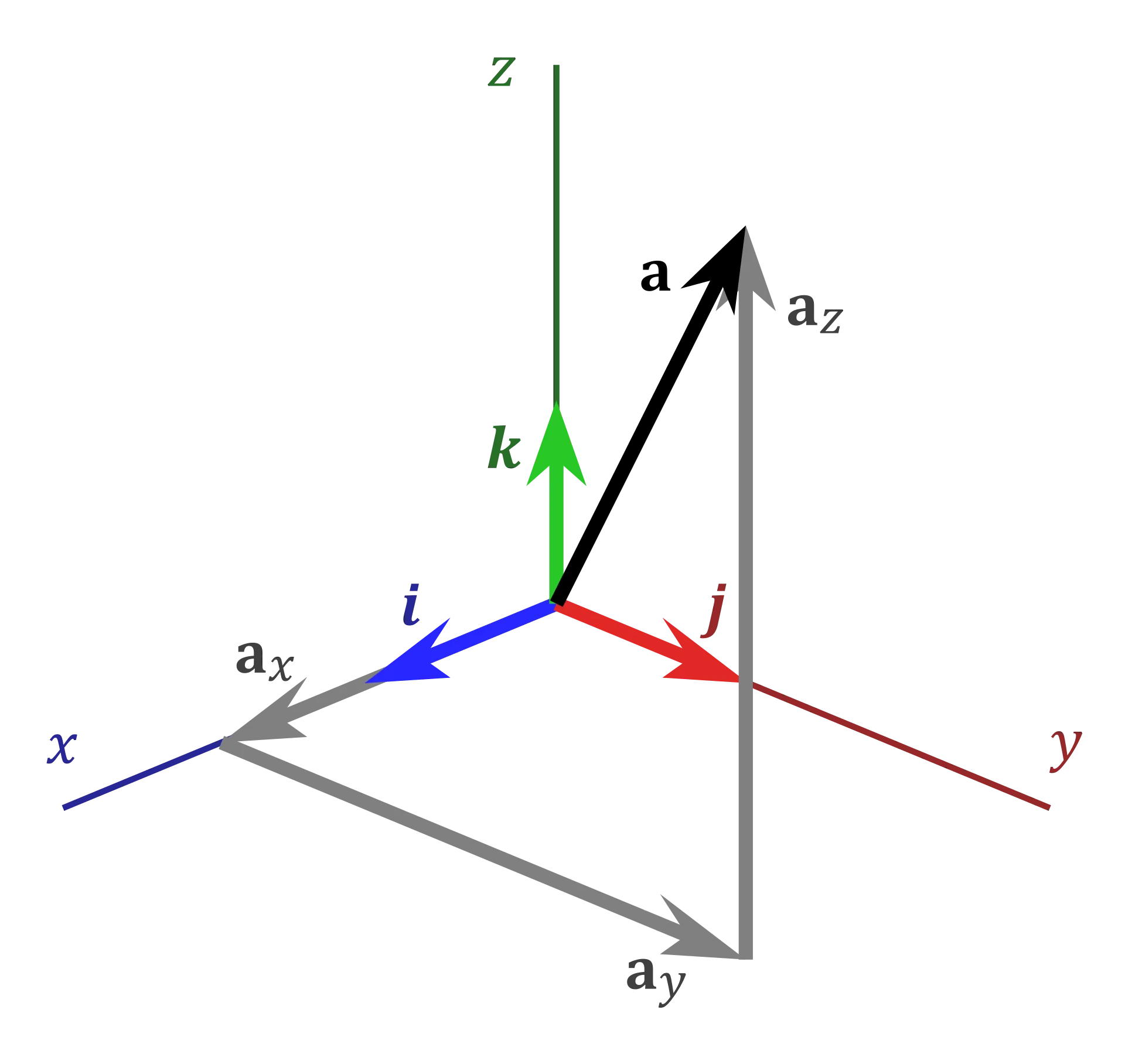
We can find a vector using the standard basis. (Source: Wikipedia)

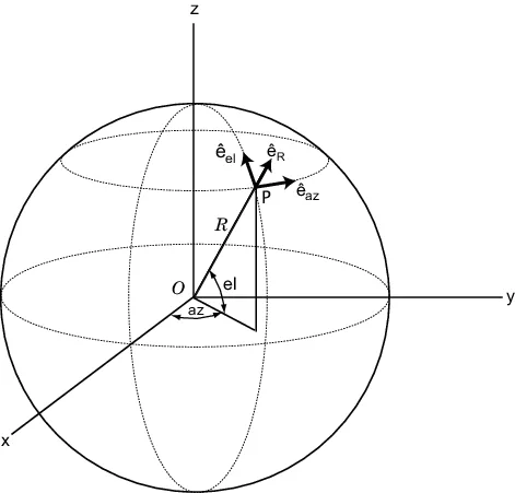
We can find the same vector using the spherical basis. — We can also find the vector using the spherical basis. (Source: MathWorks)

The fact that the representation is unique allows us to write $\vec{x}$ as an array of numbers:

$\displaystyle\vec{x} = \left[\begin{array}{c} x_{1} \\[8pt] x_{2} \\[8pt] x_{3} \end{array}\right]$

It is crucial to understand that the scalar components $x_{1},\,x_{2},\,x_{3}$ only mean something under the basis $\{\vec{e}_{1},\,\vec{e}_{2},\,\vec{e}_{3}\}$ . In other words, it is important to first agree on which basis will represent the space $\mathbb{R}^{3}$ . (Is it x, y, and z? Or radius, latitude, and longitude?)

If we choose a different basis $\{\vec{e}_{1}\,\!\!',\,\vec{e}_{2}\,\!\!',\,\vec{e}_{3}\,\!\!'\}$ , the vector $\vec{x}$ will remain the same but the scalar components $x_{1}\,\!\!',\,x_{2}\,\!\!',\,x_{3}\,\!\!'$ that represent $\vec{x}$ will be different. We write,

$\displaystyle\vec{x} = \left[\begin{array}{c} x_{1}\,\!\!' \\[8pt] x_{2}\,\!\!' \\[8pt] x_{3}\,\!\!' \end{array}\right]$

The numbers $x_{1}\,\!\!',\,x_{2}\,\!\!',\,x_{3}\,\!\!'$ , again, only mean something under the basis $\{\vec{e}_{1}\,\!\!',\,\vec{e}_{2}\,\!\!',\,\vec{e}_{3}\,\!\!'\}$ .

Later, we will show how the two sets of components $\{x_{1},\,x_{2},\,x_{3}\}$ and $\{x_{1}\,\!\!',\,x_{2}\,\!\!',\,x_{3}\,\!\!'\}$ (two coordinate systems) are related to each other. We will see that the two are related linearly through the directional cosines.

c. $\mathbb{R}^{3}$ comes with a norm and an inner product

An inner product is a function that maps a vector to a scalar. This function meets a set of requirements and, as a result, we can use numbers to describe the “geometry” of the vector space. In particular, we can talk about the length (norm) of a vector and the angle between two vectors. (On some vector spaces, we can’t define an inner product or a norm. We should be glad that both exist in $\mathbb{R}^{3}$ .)

Let $\{\vec{e}_{x},\,\vec{e}_{y},\,\vec{e}_{z}\}$ denote the standard basis for $\mathbb{R}^{3}$ . The three vectors are defined to align with the Cartesian coordinate axes in the positive directions. The components of $\vec{e}_{x},\,\vec{e}_{y},\,\vec{e}_{z}$ in terms of the standard basis (themselves) are as follows:

$\displaystyle\vec{e}_{x} = \left[\begin{array}{c} 1 \\[8pt] 0 \\[8pt] 0 \end{array}\right],\,\,\,\,\,\vec{e}_{y} = \left[\begin{array}{c} 0 \\[8pt] 1 \\[8pt] 0 \end{array}\right],\,\,\,\,\,\vec{e}_{z} = \left[\begin{array}{c} 0 \\[8pt] 0 \\[8pt] 1 \end{array}\right]$

Then, we can define an inner product between two vectors $\vec{x} = x_{1}\vec{e}_{x} + x_{2}\vec{e}_{y} + x_{3}\vec{e}_{z}$ and $\vec{y} = y_{1}\vec{e}_{x} + y_{2}\vec{e}_{y} + y_{3}\vec{e}_{z}$ as follows:

Equation 1.1. Inner product

$\displaystyle\langle\vec{x},\,\vec{y}\rangle := x_{1}y_{1} + x_{2}y_{2} + x_{3}y_{3}$

This does meet the properties of an inner product, and is called the $l^{2}$ inner product (or the Euclidean inner product) of $\vec{x}$ and $\vec{y}$ .

We can always use an inner product to define a norm, a vector-to-scalar function that measures the length of a vector. (Not all norms come from an inner product.)

Using the $l^{2}$ inner product, we define the norm of the vector $\vec{x} = x_{1}\vec{e}_{x} + x_{2}\vec{e}_{y} + x_{3}\vec{e}_{z}$ as follows:

Equation 1.2. Norm

$\displaystyle||\vec{x}||_{2} := \sqrt{\langle\vec{x},\,\vec{x}\rangle} = \sqrt{(x_{1})^{2} + (x_{2})^{2} + (x_{3})^{2}}$

This does meet the properties of a norm, and is called the $l^{2}$ norm (or the Euclidean norm) of $\vec{x}$ . We see that,

$\begin{array}{c} ||\vec{e}_{x}||_{2} = \sqrt{(1)^{2} + (0)^{2} + (0)^{2}} = 1 \\[16pt] ||\vec{e}_{y}||_{2} = \sqrt{(0)^{2} + (1)^{2} + (0)^{2}} = 1 \\[16pt] ||\vec{e}_{z}||_{2} = \sqrt{(0)^{2} + (0)^{2} + (1)^{2}} = 1 \end{array}$

i.e. the standard basis vectors have a length of 1 in the $l^{2}$ norm.

Now that we have an inner product and a norm, we can define the angle $\theta$ between two vectors $\vec{x}$ and $\vec{y}$ . We let $\theta \in [0^{\circ},\,180^{\circ}]$ be the number that satisfies the equation,

Equation 1.3. Angle

$\displaystyle\langle\vec{x},\,\vec{y}\rangle = ||\vec{x}||_{2}||\vec{y}||_{2}\cos\theta$

We say that $\vec{x}$ and $\vec{y}$ are orthogonal, or perpendicular, if $\langle\vec{x},\,\vec{y}\rangle = 0$ . From equation 1.3, we see that $\vec{x}$ and $\vec{y}$ are orthogonal when they form an angle of $90^{\circ}$ (assuming neither is the zero vector).

We can define the angle between two vectors using inner product and norm. (Source: Wikipedia)

Any two of the standard basis vectors $\vec{e}_{x},\,\vec{e}_{y},\,\vec{e}_{z}$ are orthogonal. Because they are pairwise orthogonal and have a unit length (“normalized”), we say that the standard basis is an orthonormal basis.

We defined the $l^{2}$ inner product and the $l^{2}$ norm after agreeing to use the standard basis. However, we can show that their outputs, i.e. the numbers that we get, will be the same under any orthonormal basis.

2. Coordinate Transformations

Recall that $\mathbb{R}^{3}$ is a vector space of dimension 3, so three linearly independent vectors will span the entire space. For example, we can use the standard basis $\{\vec{e}_{x},\,\vec{e}_{y},\,\vec{e}_{z}\}$ that aligns with the Cartesian coordinate system. The standard basis is an orthonormal basis, i.e. the basis vectors are pairwise orthogonal (in the sense of $l^{2}$ inner product) and have a unit length (in the sense of $l^{2}$ norm).

Remark.

As long as three vectors are linearly independent, they will form a basis of $\mathbb{R}^{3}$ . What is the benefit of considering basis vectors that are pairwise orthogonal?

a. Transforming vectors

Consider a vector $\vec{u} \in \mathbb{R}^{3}$ . We can use the standard basis to write that,

$\displaystyle\vec{u} = u_{x}\vec{e}_{x} + u_{y}\vec{e}_{y} + u_{z}\vec{e}_{z} = \left[\begin{array}{c} u_{x} \\[8pt] u_{y} \\[8pt] u_{z} \end{array}\right]$

But sometimes, it is easier to describe a structure’s behavior (e.g. displacement, reaction force) in a different coordinate system, i.e. a different basis.

Let $\{\vec{e}_{A},\,\vec{e}_{T},\,\vec{e}_{S}\}$ denote a second orthonormal basis for $\mathbb{R}^{3}$ . Note, A stands for axial, T for transverse, and S for the axis that is orthogonal to A and T.

Then, in this basis,

$\displaystyle\vec{u} = u_{A}\vec{e}_{A} + u_{T}\vec{e}_{T} + u_{S}\vec{e}_{S} = \left[\begin{array}{c} u_{A} \\[8pt] u_{T} \\[8pt] u_{S} \end{array}\right]$

We would like to know how to find the components $u_{A},\,u_{T},\,u_{S}$ under the new basis from the components $u_{x},\,u_{y},\,u_{z}$ , or vice versa. To do so, we first note that,

Equation 2.1. Identity

$\displaystyle u_{A}\vec{e}_{A} + u_{T}\vec{e}_{T} + u_{S}\vec{e}_{S} = u_{x}\vec{e}_{x} + u_{y}\vec{e}_{y} + u_{z}\vec{e}_{z}$

since both sides of the equation represent the same vector $\vec{u}$ .

The idea is to take the inner product of both sides of equation 2.1 with the new basis vectors. For example, if we take the inner product with $\vec{e}_{A}$ , we get,

$\displaystyle u_{A}\langle\vec{e}_{A},\,\vec{e}_{A}\rangle + u_{T}\langle\vec{e}_{A},\,\vec{e}_{T}\rangle + u_{S}\langle\vec{e}_{A},\,\vec{e}_{S}\rangle = u_{x}\langle\vec{e}_{A},\,\vec{e}_{x}\rangle + u_{y}\langle\vec{e}_{A},\,\vec{e}_{y}\rangle + u_{z}\langle\vec{e}_{A},\,\vec{e}_{z}\rangle$

Since $\{\vec{e}_{A},\,\vec{e}_{T},\,\vec{e}_{S}\}$ is an orthonormal basis, the equation above simply becomes,

$\displaystyle u_{A} = u_{x}\langle\vec{e}_{A},\,\vec{e}_{x}\rangle + u_{y}\langle\vec{e}_{A},\,\vec{e}_{y}\rangle + u_{z}\langle\vec{e}_{A},\,\vec{e}_{z}\rangle$

Similarly, by taking the inner product with $\vec{e}_{T}$ and with $\vec{e}_{S}$ , we get,

$\begin{array}{c} u_{T} = u_{x}\langle\vec{e}_{T},\,\vec{e}_{x}\rangle + u_{y}\langle\vec{e}_{T},\,\vec{e}_{y}\rangle + u_{z}\langle\vec{e}_{T},\,\vec{e}_{z}\rangle \\[16pt] u_{S} = u_{x}\langle\vec{e}_{S},\,\vec{e}_{x}\rangle + u_{y}\langle\vec{e}_{S},\,\vec{e}_{y}\rangle + u_{z}\langle\vec{e}_{S},\,\vec{e}_{z}\rangle \end{array}$

Remark.

The idea of using consistent nodal forces to approximate a distributed load relies on inner products. In some sense, nodal forces represent one coordinate system, and distributed loads represent another.

We can combine these three equations into a single matrix equation:

Equation 2.2.

$\displaystyle \left[\begin{array}{c} u_{A} \\[8pt] u_{T} \\[8pt] u_{S} \end{array}\right] = \underbrace{\left[\begin{array}{ccc} \langle\vec{e}_{A},\,\vec{e}_{x}\rangle & \langle\vec{e}_{A},\,\vec{e}_{y}\rangle & \langle\vec{e}_{A},\,\vec{e}_{z}\rangle \\[8pt] \langle\vec{e}_{T},\,\vec{e}_{x}\rangle & \langle\vec{e}_{T},\,\vec{e}_{y}\rangle & \langle\vec{e}_{T},\,\vec{e}_{z}\rangle \\[8pt] \langle\vec{e}_{S},\,\vec{e}_{x}\rangle & \langle\vec{e}_{S},\,\vec{e}_{y}\rangle & \langle\vec{e}_{S},\,\vec{e}_{z}\rangle \end{array}\right]}_{:=\,Q}\left[\begin{array}{c} u_{x} \\[8pt] u_{y} \\[8pt] u_{z} \end{array}\right]$

Hence, we can change the components of $\vec{u}$ from one coordinate system to a new one by applying a linear transformation $Q$ :

Equation 2.3.

$\displaystyle \vec{u}_{\mbox{\tiny new}} = Q\vec{u}$

Note that, by the angle formula (equation 1.3), we can interpret each inner product $\langle\vec{e}_{i},\,\vec{e}_{j}\rangle$ as the cosine of the angle between two coordinate axes $\vec{e}_{i}$ and $\vec{e}_{j}$ :

$\displaystyle Q = \left[\begin{array}{ccc} \cos\theta_{Ax} & \cos\theta_{Ay} & \cos\theta_{Az} \\[8pt] \cos\theta_{Tx} & \cos\theta_{Ty} & \cos\theta_{Tz} \\[8pt] \cos\theta_{Sx} & \cos\theta_{Sy} & \cos\theta_{Sz} \end{array}\right]$

We call these cosines, the directional cosines.

We can also show that $Q$ is an orthogonal matrix. This means $Q$ is invertible and its inverse is easily given by the transpose matrix, i.e. $Q^{-1} = Q^{T}$ .

Hence, we can find $u_{x},\,u_{y},\,u_{z}$ from $u_{A},\,u_{T},\,u_{S}$ :

Equation 2.4.

$\displaystyle\vec{u} = Q^{T}\vec{u}_{\mbox{\tiny new}}$

b. Transforming matrices

A matrix $A \in \mathbb{R}^{3 \times 3}$ can be represented by nine components. Again, we would like to know how these components will change under a new basis (basis for matrices $\mathbb{R}^{3 \times 3}$ ). This would be useful for computing an element stiffness matrix and for describing the strains and stresses within the structure. While it is possible to come up with a basis and an inner product for matrices and repeat what we just did for vectors, there is an easier way to arrive at the result.

We use the fact that a matrix $A \in \mathbb{R}^{3 \times 3}$ linearly maps vectors in $\mathbb{R}^{3}$ to vectors in $\mathbb{R}^{3}$ . In other words, $A$ allows the equation,

$\displaystyle A\vec{u} = \vec{b}$

From equation 2.3, we know how the components of a vector change under a new basis for $\mathbb{R}^{3}$ . Let $\vec{u}_{\mbox{\tiny new}} = Q\vec{u}$ and $\vec{b}_{\mbox{\tiny new}} = Q\vec{b}$ denote the components of $\vec{u}$ and $\vec{b}$ in the new basis. Substitute these relations into the equation above (recall, $Q$ is orthogonal) to find that,

$\displaystyle QAQ^{T}\vec{u}_{\mbox{\tiny new}} = \vec{b}_{\mbox{\tiny new}}$

Because this equation holds for all vectors $\vec{u}$ and $\vec{b}$ (that satisfied the original equation), we can conclude that $A_{\mbox{\tiny new}}$ , the components of the matrix in the new basis, is given by,

Equation 2.5.

$\displaystyle A_{\mbox{\tiny new}} = QAQ^{T}$

Notice the similarity and dissimilarity between the transformation rules for vectors (equation 2.3) and for matrices (equation 2.5).

3. Applications

a. Element stiffness matrix of 2D and 3D truss elements

Consider the element stiffness matrix for a 2D truss element. Locally (in axial and transversal directions), the element stiffness matrix is very easy to describe:

$\displaystyle K^{e}_{\mbox{\tiny local}} = \frac{EA}{L}\left[\begin{array}{cccc} 1 & 0 & -1 & 0 \\[8pt] 0 & 0 & 0 & 0 \\[8pt] -1 & 0 & 1 & 0 \\[8pt] 0 & 0 & 0 & 0 \end{array}\right]$

To study how all 2D truss elements interact with each other (and possibly with other types of elements), we need to convert this local element stiffness matrix to a global one. For each 2D truss element, we get to apply a change of coordinates to two nodes (i.e. two vectors in $\mathbb{R}^{2}$ ). Therefore, the transformation matrix $Q$ is a block diagonal matrix as shown below:

$\displaystyle Q = \left[\begin{array}{cccc} \cos\theta_{Ax} & \cos\theta_{Ay} & 0 & 0 \\[8pt] \cos\theta_{Tx} & \cos\theta_{Ty} & 0 & 0 \\[8pt] 0 & 0 & \cos\theta_{Ax} & \cos\theta_{Ay} \\[8pt] 0 & 0 & \cos\theta_{Tx} & \cos\theta_{Ty} \end{array}\right]$

Hence, the components of the element stiffness matrix in the global coordinate system (Cartesian) are given by,

$\displaystyle K^{e}_{\mbox{\tiny global}} = Q^{T}K^{e}_{\mbox{\tiny local}}Q$

We can show that the product simplifies to,

$\displaystyle K^{e}_{\mbox{\tiny global}} = \frac{EA}{L}\left[\begin{array}{cccc} \cos^{2}\theta_{Ax} & \cos\theta_{Ax}\cos\theta_{Ay} & -\cos^{2}\theta_{Ax} & -\cos\theta_{Ax}\cos\theta_{Ay} \\[8pt] \cos\theta_{Ax}\cos\theta_{Ay} & \cos^{2}\theta_{Ay} & -\cos\theta_{Ax}\cos\theta_{Ay} & -\cos^{2}\theta_{Ay} \\[8pt] -\cos^{2}\theta_{Ax} & -\cos\theta_{Ax}\cos\theta_{Ay} & \cos^{2}\theta_{Ax} & \cos\theta_{Ax}\cos\theta_{Ay} \\[8pt] -\cos\theta_{Ax}\cos\theta_{Ay} & -\cos^{2}\theta_{Ay} & \cos\theta_{Ax}\cos\theta_{Ay} & \cos^{2}\theta_{Ay} \end{array}\right]$

This element stiffness matrix is the same as that given in Topics in Computational Mechanics: Part 1, with $\cos\theta_{Ax} \equiv \cos\theta$ and $\cos\theta_{Ay} \equiv \sin\theta$ .

Remark.

How will the element stiffness matrix for a 3D truss element look like in the global coordinate system?

b. Axial strain in 2D and 3D truss elements

We define the axial strain $\varepsilon_{A}$ to be the relative change in the length of a truss. Locally, this is very easy to describe using axial displacements (1 and 2 are node indices):

$\displaystyle\varepsilon_{A} = \frac{u_{2,A} - u_{1,A}}{L}$

Recall the relation between axial displacement and the global displacements,

$\displaystyle u_{A} = u_{x}\cos\theta_{Ax} + u_{y}\cos\theta_{Ay} + u_{z}\cos\theta_{Az}$

Hence, we can find the axial strain from the global displacements using directional cosines:

$\displaystyle\varepsilon_{A} = \Bigl(\frac{u_{2,x} - u_{1,x}}{L}\Bigr)\cos\theta_{Ax} + \Bigl(\frac{u_{2,y} - u_{1,y}}{L}\Bigr)\cos\theta_{Ay} + \Bigl(\frac{u_{2,z} - u_{1,z}}{L}\Bigr)\cos\theta_{Az}$