Over the next few posts, I will share the writings and programs that I had created for a class in computational structural analysis—how we efficiently analyze a structure using numerical methods. The field is a subset of computational mechanics, which combines the disciplines of mathematics, computer science, and engineering.
The class consisted of juniors and seniors in mechanical or aerospace engineering. In other words, for brevity, I will assume that you have some familiarity with statics, linear algebra, and calculus. If time permits in future, I will upload my class notes to fill gaps and share more drawings.
1. Definitions
We will be looking at bars, beams, trusses, and frames. These are structures that we classify according to what they can and cannot do.
A bar represents a 1D structural element that can withstand only axial forces—tensile or compressive forces directed along the element's local (reference) axis. We assume that a bar cannot carry other types of internal forces, such as shear force, bending moment, and twisting moment. A bar is the simplest 1D element, but it can also show complex behavior such as buckling.
A beam represents a 1D element that can withstand not only axial forces (tensile or compressive), but also an internal force that involves transverse shear force, bending moment, and twisting moment. As you can imagine, a beam is more complex than a bar, both physically and mathematically.
We can join 1D elements such as bars and beams to form a complex 3D structure. A truss is a structure where the predominant behavior of each element is axial force transmission (bar-like). If some of the elements in a structure carry loads such that internal forces and/or internal moments exist (beam-like), then we refer to the structure as a frame.
2. Truss Examples
What better way to learn than solving problems by hand?
I had created 3 problems for my recitation. Each is challenging as we allow arbitrary parameters that meet small-strain constraint. The last two problems also mark an important lesson in computational mechanics: whenever possible, choose an easy coordinate system and use symmetry to simplify a problem.
a. Assembly of truss
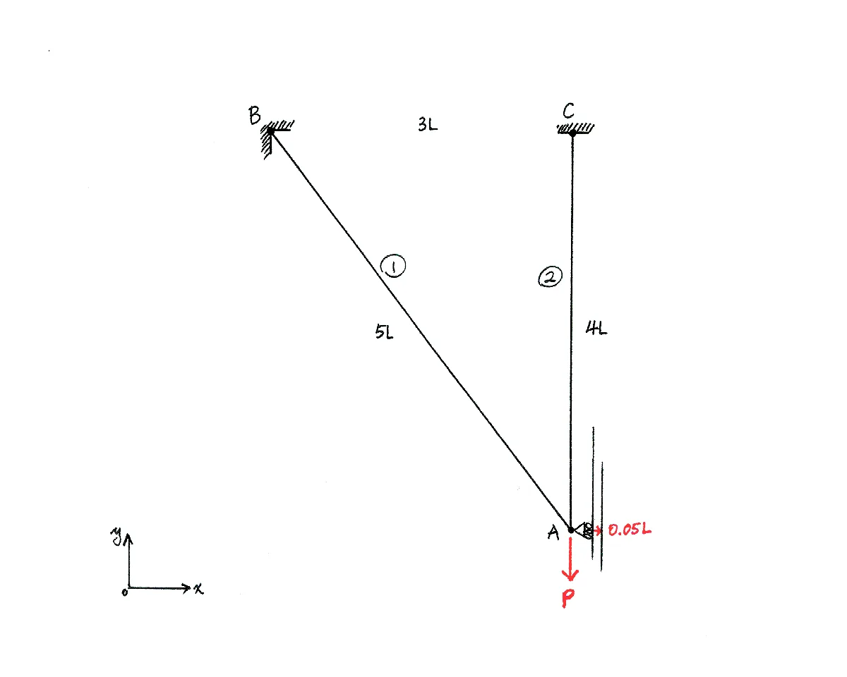
Consider a truss with two bars, one of length 5L and the other 4L. The bars are joined by a roller at node A, while their other ends are fixed, as shown below:
A two-bar truss with horizontal displacement and vertical load applied to node A.
A force of P is applied to node A in the negative y direction, while node A moves by an amount of 0.05L in the positive x direction. Both bars are assumed to be linearly elastic and isotropic, with Young's modulus E and cross-sectional area A.
Determine the y displacement of node A and the axial force in each bar. For a model problem, we can use the following parameters:
P=106NL=1mE=210GPa(steel)A=5×10⁻⁴m2(5cm2)
i. Notations
First, let's agree on our notations. We will write the displacements of the nodes (also called degrees of freedom) as,
uA,x,uA,y,uB,x,uB,y,uC,x,uC,y
the bars' internal forces as,
f1,f2
and the reaction forces as,
fA,x,fA,y,fB,x,fB,y,fC,x,fC,y
ii. Equilibrium equations
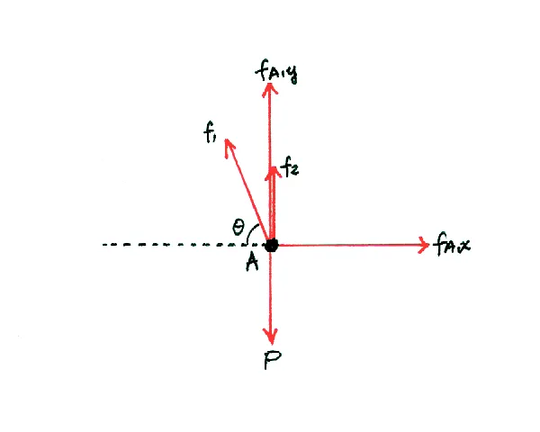
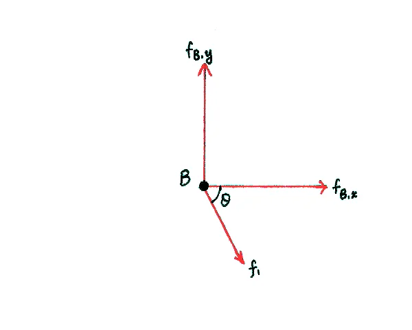
The net forces along x and y directions must be 0. To help us derive the equilibrium equations, we will draw free-body diagrams for each node.
Free-body diagram for node A
Free-body diagram for node B
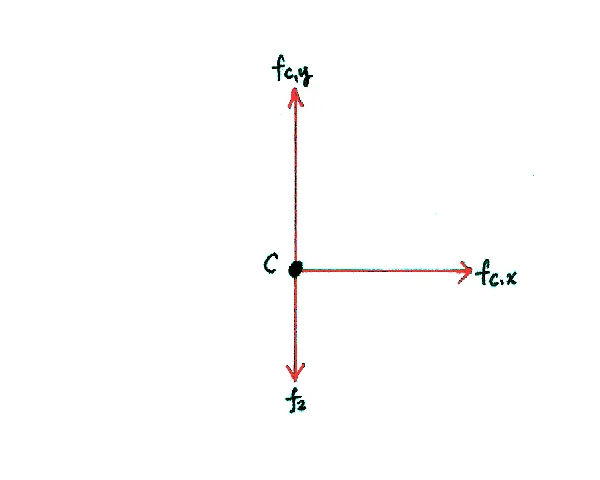
Free-body diagram for node C
For node A, we get the following system of equations:
−53f1+fA,x54f1+f2+fA,y−P==00
For node B,
53f1+fB,x−54f1+fB,y==00
Finally, for node C,
fC,x−f2+fC,y==00
We can combine these equations into a single matrix equation:
The matrix K∈R6×6 is called the stiffness matrix. It represents the relation between the nodal displacements and internal forces.
From above, we see that the first two columns of K are linearly independent. On the other hand, each of the remaining four columns can be written as a linear combination of these two. Hence, rank(K)=2.
This means, we need to specify (at least) 4 displacement constraints in order to get a unique solution.
v. Boundary conditions
From the problem description, we know that,
uA,x=0.05LuB,x,uB,y,uC,x,uC,y=0fA,y=0
We can find the y displacement of node A from the second equation:
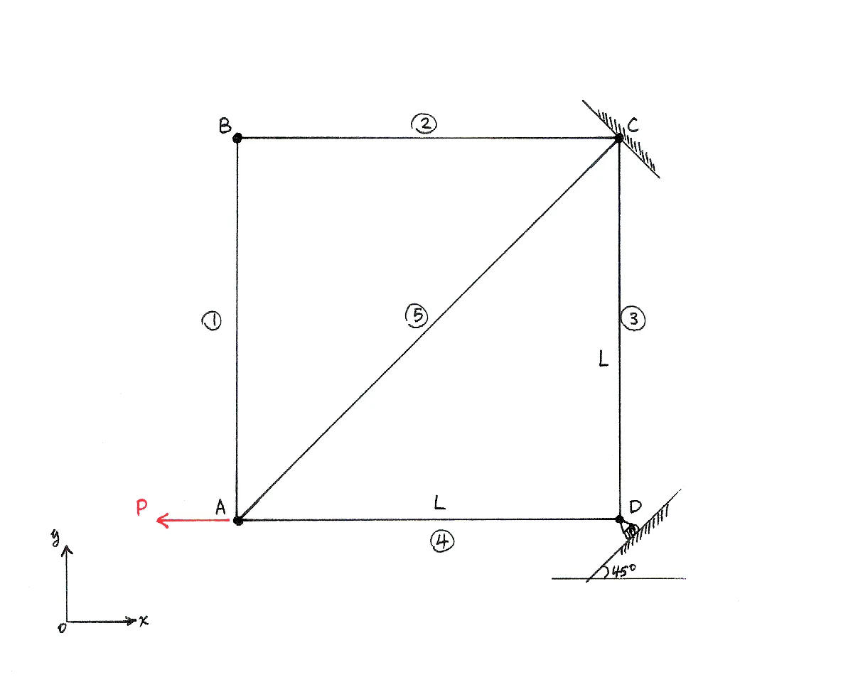
Consider a truss with 5 bars. All bars are linearly elastic and isotropic, with Young's modulus E and cross-sectional area A.
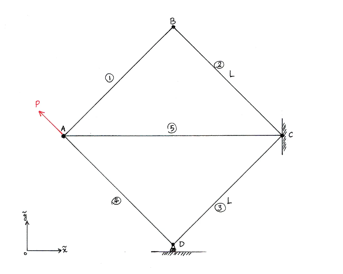
A five-bar truss with horizontal load applied to node A.
A force of P is applied to node A in the negative x direction. Notice that node D is on a roller that is inclined at an angle of 45∘.
Find the unknown displacements. Then, determine which bars increase in length, decrease, or remain the same.
i. Element stiffness matrices
Rather than deriving the equilibrium, stress-strain, and strain-displacement equations again, we can compute the element stiffness matrixKe for each bar and assemble the element matrices (stitch them together, so to speak) to create the stiffness matrix K.
For a bar with nodes i and j, its element stiffness matrix is given by,
The angle θ measures the rotation that the bar needs to align with the global x–y coordinate system.
There is an easy visual trick that I use to correctly determine θ. Take the positive x axis—in particular, I think of a vector pointing to the right—and rotate it until it matches the vector that points from node i to node j. The amount of rotation needed is θ. From this, we can compute the cosine and sine values.
For bar element 1, which goes from node A to B, we have cosθ=0 and sinθ=1.
Note that rank(K)=5, so we must have at least 3 displacement constraints in order to get a unique solution.
iii. Boundary conditions
From the drawing in the beginning, we can easily see that,
uC,x,uC,y=0fA,x,fA,y,fB,x,fB,y=0
There is a duality between known displacements and unknown forces (and vice versa). We know the displacements of node C, but don't know its reaction forces. We know the reaction forces of nodes A and B, but don't know their displacements.
We have 2 displacement constraints and need 1 more to find a unique solution. What about node D, which moves along the inclined plane?
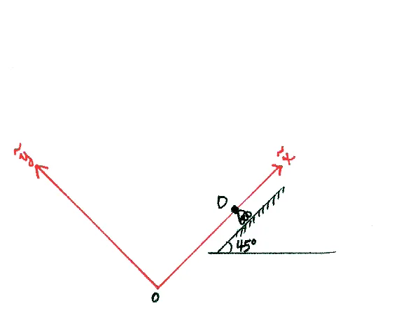
Consider a local coordinate system at node D. This means, one of the axes is parallel to the inclined plane. Since the node's expected movement matches one of the axes, it will be easier to describe the displacement of node D.
A local coordinate system at node D.
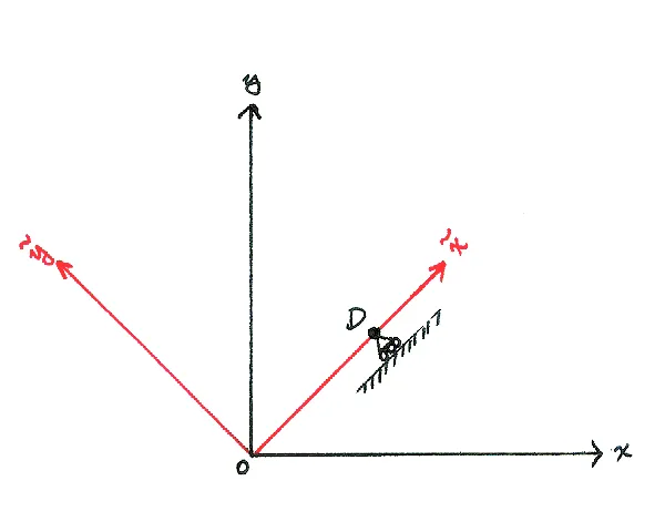
Without loss of generality, we can assume that the local coordinate system (x~,y~) shares the same origin as the global coordinate system (x,y).
The local coordinate system shares the same origin as the global.
Our goal is to describe the displacement of node D in the local coordinate system. Keep in mind that the act of displacement is the same whether we consider global or local coordinates, but the numbers representing the displacement depend on which coordinate system we consider. More precisely, they depend on which basis we consider to represent the space of R2.
The basis for the local coordinate system, in terms of the global coordinates (the standard basis), is given by,
Note that the 5th entry of freduced, which had been fD,x, was changed to −(EA/L)uD,x. Since the variable uD,x is unknown, the coefficient −(EA/L) moved to the left-hand side of the equation. This is how we get the coefficient of 2 on row 5, column 5 of the matrix Kreduced.
Solve for the vector ureduced.
uA,xuA,yuB,xuB,yuD,x=EAPL−2202−1
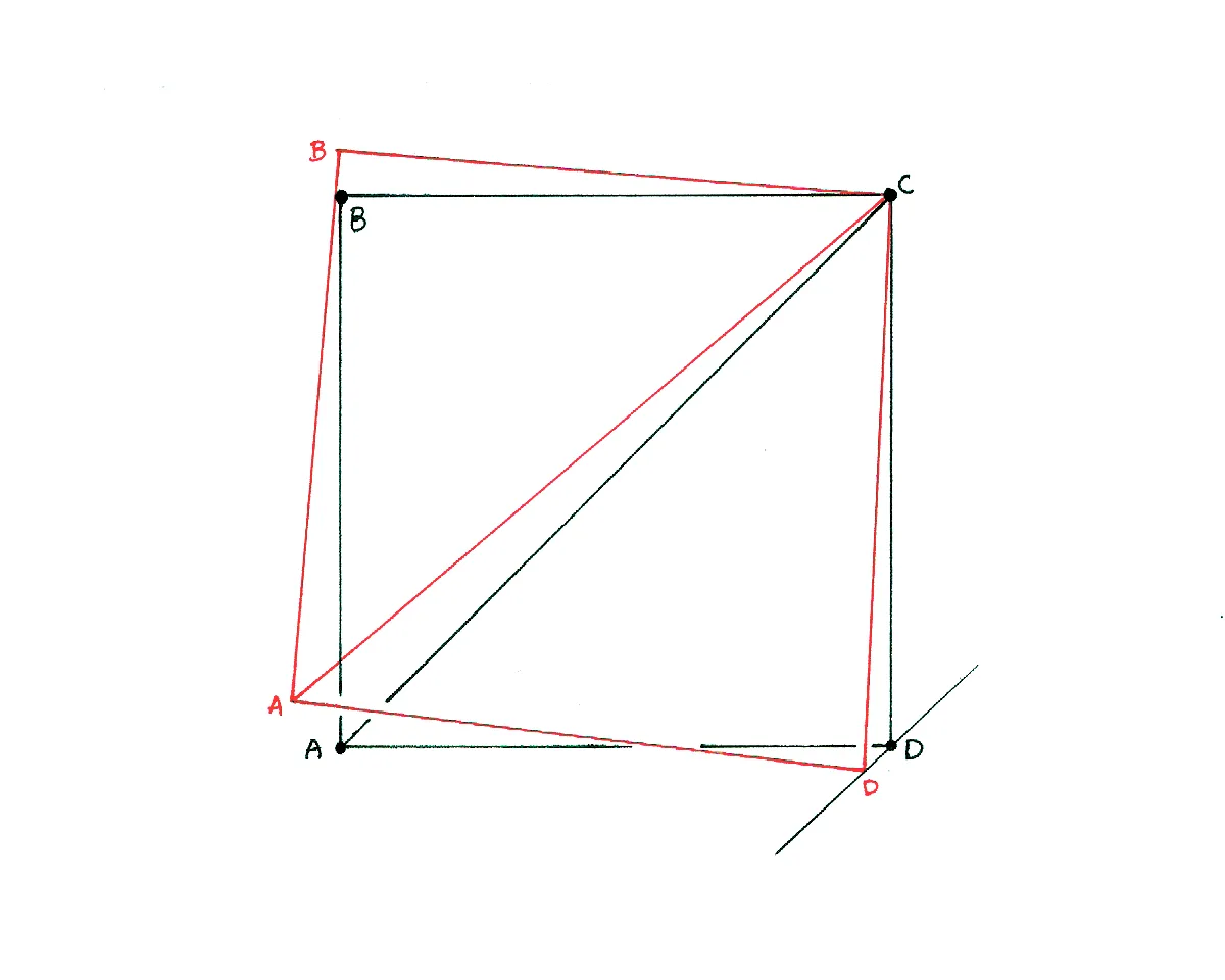
Since we know the displacements, we can visualize the deformed structure:
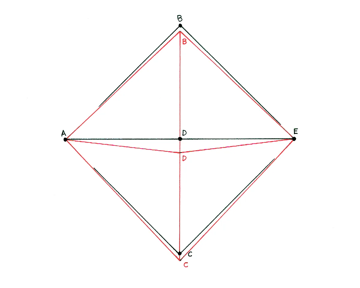
Before and after the deformation.
v. Postprocessing
Once we have the displacements, we can calculate the strains (if desired, stresses too) in each bar.
From these strains, we can feel the deformed geometry. Since bar 5 (the diagonal one) did not change in length while bars 3 and 4 increased in length, the angle between bars 3 and 4 must have decreased. Bars 1 and 2 are simply lifted up.
vi. Remarks
There is an easier way to solve this problem. We recall that the difficulty of solving it came from determining the boundary condition at node D.
What if, instead, we consider the following coordinate system (tilt our head by 45∘)?
The same problem in a different coordinate system.
The roller BC becomes much easier to derive now.
u~D,y=0f~D,x=0
c. Effect of symmetry
Last but not least, let's look at how to simplify a problem when there is symmetry in the structure and boundary conditions.
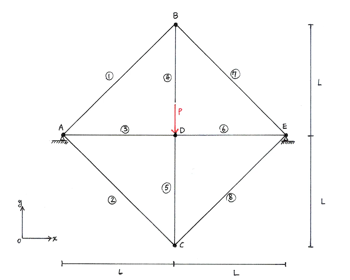
A 8-bar truss that exhibits symmetry.
As usual, all bars are linearly elastic and isotropic. To make our hand calculations easy, we assign the material parameters E and 2A to bars 1, 2, 7, and 8, and parameters of E and A to bars 3, 4, 5, and 6.
With this setup, the truss exhibits symmetry about the line BC, i.e. identical geometry, material, loading, and displacements occur on each side about this line.
When there is symmetry, we can reduce the problem by following these steps:
For loads that occur in the plane of symmetry, apply half of the total load to the reduced structure.
For elements in the plane of symmetry, take half of the cross-sectional area.
For nodes in the plane of symmetry, the displacement components that are normal (perpendicular) to the plane of symmetry must be set to 0.
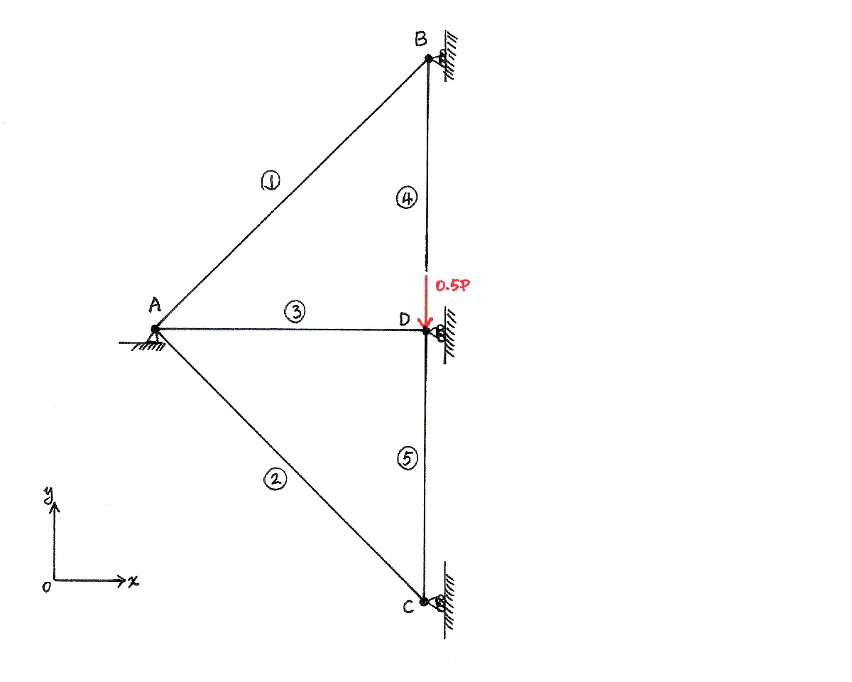
Now, we can solve a simpler problem:
Use symmetry to reduce the number of unknowns (degrees of freedom).
Note that bars 4 and 5 now have the (effective) cross-sectional area 0.5A.
i. Element stiffness matrices
For element 1 (node A to B), cosθ=21 and sinθ=21.
Hence, the structure deforms in the following manner:
Before and after the deformation.
v. Remarks
As we saw from above, symmetry helps us simplify a problem. For structural problems in 2D or 3D, reducing the number of unknowns (DOFs) can have a significant positive impact on speed and accuracy.
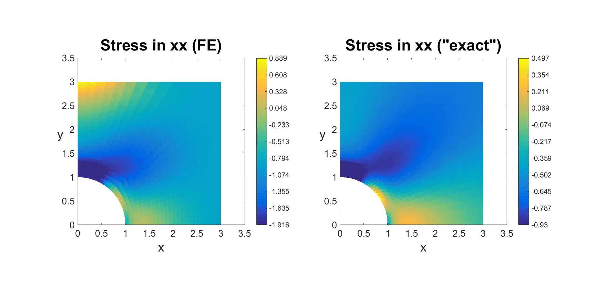
A classic example is the infinite plate with a circular hole that goes under uniaxial or biaxial tension. For this problem, we just need to model a quarter of the geometry.
Stress distribution for a finite plate with a circular hole.