← Back to Home

Iterative Methods: Part 3

Let's look at one more way to solve the equation Ax⃗=b⃗A\vec{x} = \vec{b}. We assume that A∈Rn×nA \in \mathbb{R}^{n \times n} is nonsingular, and define the kk-th Krylov subspace as follows:

Kk := span{b⃗, Ab⃗, ⋯ , Ak−1b⃗}.\mathscr{K}_{k} \,:=\, \text{span}\{\vec{b},\,A\vec{b},\,\cdots,\,A^{k - 1}\vec{b}\}.

Krylov subspace methods are efficient and popular iterative methods for solving large, sparse linear systems. When AA is symmetric, positive definite (SPD), i.e.

{AT=Ax⃗TAx⃗>0,   ∀ x⃗≠0⃗,\left\{\begin{array}{l} A^{T} = A \\ \vec{x}^{T}A\vec{x} > 0,\,\,\,\forall\,\vec{x} \neq \vec{0}, \end{array}\right.

we can use a Krylov subspace method called Conjugate Gradient (CG).

Today, let's find out how CG works and use it to solve 2D Poisson's equation.

4. Conjugate Gradient

a. Creating iterates

Let (⋅, ⋅)(\cdot,\,\cdot) be an inner product for Rn\mathbb{R}^{n}, and ∣∣⋅∣∣:=(⋅, ⋅)||\cdot|| := \sqrt{(\cdot,\,\cdot)} the norm associated with the inner product.

How Krylov subspace methods work is simple. We will approximate the exact solution x⃗=A−1b⃗\vec{x} = A^{-1}\vec{b} with a sequence of iterates x⃗k\vec{x}_{k} that meet two conditions:

1.   x⃗k∈Kk2.   ∣∣x⃗k−x⃗∣∣=min⁡y⃗ ∈ Kk ∣∣y⃗−x⃗∣∣.\begin{array}{l} \text{1.}\,\,\,\vec{x}_{k} \in \mathscr{K}_{k} \\ \text{2.}\,\,\,||\vec{x}_{k} - \vec{x}|| = \min\limits_{\vec{y}\,\in\,\mathscr{K}_{k}}\,||\vec{y} - \vec{x}||. \end{array}

In other words, when measured in the norm ∣∣⋅∣∣||\cdot||, x⃗k\vec{x}_{k} is the best approximation to x⃗\vec{x} from the kk-th Krylov subspace.

(For initialization, we will take x⃗0=0⃗\vec{x}_{0} = \vec{0} and K0={0⃗}\mathscr{K}_{0} = \{\vec{0}\}.)

The optimality condition above is the same as the orthogonality condition x⃗k−x⃗⊥Kk\vec{x}_{k} - \vec{x} \perp \mathscr{K}_{k} under the inner product (⋅, ⋅)(\cdot,\,\cdot). Therefore, x⃗k\vec{x}_{k} satisfies the equation,

(x⃗k−x⃗, y⃗)=0,   ∀ y⃗∈Kk.(\vec{x}_{k} - \vec{x},\,\vec{y}) = 0,\,\,\,\forall\,\vec{y} \in \mathscr{K}_{k}.

Lemma 1.

The orthogonality condition and the fact that Kk−1⊂Kk\mathscr{K}_{k - 1} \subset \mathscr{K}_{k} imply two things. At every iteration k≥1k \geq 1,

1.   x⃗k−x⃗k−1∈Kk2.   x⃗k−x⃗k−1⊥Kk−1.\begin{array}{l} \text{1.}\,\,\,\vec{x}_{k} - \vec{x}_{k - 1} \in \mathscr{K}_{k} \\ \text{2.}\,\,\,\vec{x}_{k} - \vec{x}_{k - 1} \perp \mathscr{K}_{k - 1}. \end{array}

Proof.

First, note that the vector

x⃗k−x⃗k−1 ≡ (x⃗k−x⃗)−(x⃗k−1−x⃗)\vec{x}_{k} - \vec{x}_{k - 1} \,\equiv\, (\vec{x}_{k} - \vec{x}) - (\vec{x}_{k - 1} - \vec{x})

represents the decrease in error over 1 iteration.

Since x⃗k∈Kk\vec{x}_{k} \in \mathscr{K}_{k} and x⃗k−1∈Kk−1⊂Kk\vec{x}_{k - 1} \in \mathscr{K}_{k - 1} \subset \mathscr{K}_{k}, we know that x⃗k−x⃗k−1∈Kk\vec{x}_{k} - \vec{x}_{k - 1} \in \mathscr{K}_{k}.

Furthermore, for any y⃗∈Kk−1 (⊂Kk)\vec{y} \in \mathscr{K}_{k - 1}\,(\subset \mathscr{K}_{k}),

(x⃗k−x⃗k−1, y⃗) = (x⃗k−x⃗, y⃗)⏟= 0 − (x⃗k−1−x⃗, y⃗)⏟= 0 = 0.(\vec{x}_{k} - \vec{x}_{k - 1},\,\vec{y}) \,=\, \underbrace{(\vec{x}_{k} - \vec{x},\,\vec{y})}_{=\,0} \,-\, \underbrace{(\vec{x}_{k - 1} - \vec{x},\,\vec{y})}_{=\,0} \,=\, 0.

■

b. Creating residuals

Next, we select a vector p⃗k≠0⃗\vec{p}_{k} \neq \vec{0} that meets these conditions:

1.   p⃗k∈Kk2.   p⃗k⊥Kk−1.\begin{array}{l} \text{1.}\,\,\,\vec{p}_{k} \in \mathscr{K}_{k} \\ \text{2.}\,\,\,\vec{p}_{k} \perp \mathscr{K}_{k - 1}. \end{array}

(For initialization, we will take p⃗1=b⃗\vec{p}_{1} = \vec{b}.)

The vector x⃗k−x⃗k−1\vec{x}_{k} - \vec{x}_{k - 1} also satisfied these conditions, so the two are linearly dependent. There is some constant αk∈R \ {0}\alpha_{k} \in \mathbb{R}\,\backslash\,\{0\} such that x⃗k−x⃗k−1=αkp⃗k\vec{x}_{k} - \vec{x}_{k - 1} = \alpha_{k}\vec{p}_{k}.

We now have a way to compute the best approximation x⃗k\vec{x}_{k} from the previous one:

x⃗k=x⃗k−1+αkp⃗k,   ∀ k≥1.\boxed{\vec{x}_{k} = \vec{x}_{k - 1} + \alpha_{k}\vec{p}_{k},\,\,\,\forall\,k \geq 1}.

This holds, provided we have a search direction p⃗k\vec{p}_{k}.

Lemma 2.

The coefficient αk\alpha_{k} is given by,

αk=−(x⃗k−1−x⃗, p⃗k)(p⃗k, p⃗k)=(A−1r⃗k−1, p⃗k)(p⃗k, p⃗k),   ∀ k≥1,\boxed{\displaystyle\alpha_{k} = -\frac{(\vec{x}_{k - 1} - \vec{x},\,\vec{p}_{k})}{(\vec{p}_{k},\,\vec{p}_{k})} = \frac{(A^{-1}\vec{r}_{k - 1},\,\vec{p}_{k})}{(\vec{p}_{k},\,\vec{p}_{k})},\,\,\,\forall\,k \geq 1},

where r⃗k:=b⃗−Ax⃗k\vec{r}_{k} := \vec{b} - A\vec{x}_{k} is the residual.

Proof.

We have the equation,

x⃗k−x⃗=(x⃗k−1−x⃗)+αkp⃗k.\vec{x}_{k} - \vec{x} = (\vec{x}_{k - 1} - \vec{x}) + \alpha_{k}\vec{p}_{k}.

On each side, take the inner product with p⃗k\vec{p}_{k}:

(x⃗k−x⃗, p⃗k)=(x⃗k−1−x⃗, p⃗k)+αk(p⃗k, p⃗k).(\vec{x}_{k} - \vec{x},\,\vec{p}_{k}) = (\vec{x}_{k - 1} - \vec{x},\,\vec{p}_{k}) + \alpha_{k}(\vec{p}_{k},\,\vec{p}_{k}).

Since x⃗k−x⃗⊥Kk\vec{x}_{k} - \vec{x} \perp \mathscr{K}_{k} and p⃗k∈Kk\vec{p}_{k} \in \mathscr{K}_{k}, the LHS is equal to 0. Hence,

αk=−(x⃗k−1−x⃗, p⃗k)(p⃗k, p⃗k).\displaystyle\alpha_{k} = -\frac{(\vec{x}_{k - 1} - \vec{x},\,\vec{p}_{k})}{(\vec{p}_{k},\,\vec{p}_{k})}.

Note, r⃗k−1=A(x⃗−x⃗k−1)\vec{r}_{k - 1} = A(\vec{x} - \vec{x}_{k - 1}).

■

Lemma 3.

The residuals are related in the following manner:

r⃗k=r⃗k−1−αkAp⃗k,   ∀ k≥1.\boxed{\vec{r}_{k} = \vec{r}_{k - 1} - \alpha_{k}A\vec{p}_{k},\,\,\,\forall\,k \geq 1}.

Proof.

Apply AA to both sides of the equation:

(x⃗−x⃗k)=(x⃗−x⃗k−1)−αkp⃗k.(\vec{x} - \vec{x}_{k}) = (\vec{x} - \vec{x}_{k - 1}) - \alpha_{k}\vec{p}_{k}.

■

c. Creating search directions

We will now construct the search direction p⃗k+1\vec{p}_{k + 1} so that we can continue the iteration. Along the way, we required the search directions to satisfy,

p⃗i∈Ki \ {0⃗}   and   p⃗i⊥Ki−1,   ∀ i=1, ⋯ , k.\vec{p}_{i} \in \mathscr{K}_{i} \,\backslash\, \{\vec{0}\} \,\,\,\text{and}\,\,\,\vec{p}_{i} \perp \mathscr{K}_{i - 1},\,\,\,\forall\,i = 1,\,\cdots,\,k.

Thus, if p⃗k+1\vec{p}_{k + 1} also meets these conditions, namely,

p⃗k+1∈Kk+1 \ {0⃗}   and   p⃗k+1⊥Kk,\vec{p}_{k + 1} \in \mathscr{K}_{k + 1} \,\backslash\, \{\vec{0}\} \,\,\,\text{and}\,\,\,\vec{p}_{k + 1} \perp \mathscr{K}_{k},

then {p⃗1, ⋯ , p⃗k+1}\{\vec{p}_{1},\,\cdots,\,\vec{p}_{k + 1}\} will end up forming an orthogonal basis for Kk+1\mathscr{K}_{k + 1}.

We can create such a sequence using Gram-Schmidt method! Specifically, p⃗k+1\vec{p}_{k + 1} will be the sum of a vector in Kk\mathscr{K}_{k} (which can be written as a linear combination of p⃗1, ⋯ , p⃗k\vec{p}_{1},\,\cdots,\,\vec{p}_{k}) and an offshoot w⃗k∈Kk+1 \ Kk\vec{w}_{k} \in \mathscr{K}_{k + 1} \,\backslash\, \mathscr{K}_{k}:

p⃗k+1=w⃗k+∑i = 1k γip⃗i,   ∀ k≥1.\boxed{\displaystyle\vec{p}_{k + 1} = \vec{w}_{k} + \sum_{i\,=\,1}^{k}\,\gamma_{i}\vec{p}_{i},\,\,\,\forall\,k \geq 1}.

Then, we orthogonalize p⃗k+1\vec{p}_{k + 1} against p⃗1, ⋯ , p⃗k\vec{p}_{1},\,\cdots,\,\vec{p}_{k}.

Lemma 4.

In the kk-th iteration, the coefficients γi\gamma_{i} are given by,

γi=−(w⃗k, p⃗i)(p⃗i, p⃗i),   ∀ i=1, ⋯ , k.\boxed{\displaystyle\gamma_{i} = -\frac{(\vec{w}_{k},\,\vec{p}_{i})}{(\vec{p}_{i},\,\vec{p}_{i})},\,\,\,\forall\,i = 1,\,\cdots,\,k}.

Proof.

Given the equation,

p⃗k+1=w⃗k+∑j = 1k γjp⃗j,\displaystyle\vec{p}_{k + 1} = \vec{w}_{k} + \sum_{j\,=\,1}^{k}\,\gamma_{j}\vec{p}_{j},

we can take the inner product with p⃗i\vec{p}_{i}:

(p⃗k+1, p⃗i)=(w⃗k, p⃗i)+∑j = 1k γj(p⃗j, p⃗i).\displaystyle(\vec{p}_{k + 1},\,\vec{p}_{i}) = (\vec{w}_{k},\,\vec{p}_{i}) + \sum_{j\,=\,1}^{k}\,\gamma_{j}(\vec{p}_{j},\,\vec{p}_{i}).

Since p⃗k+1⊥Ki\vec{p}_{k + 1} \perp \mathscr{K}_{i} and p⃗i∈Ki\vec{p}_{i} \in \mathscr{K}_{i}, the LHS is equal to 0. Furthermore, {p⃗1, ⋯ , p⃗k}\{\vec{p}_{1},\,\cdots,\,\vec{p}_{k}\} forms an orthogonal basis, so the summation on the RHS reduces to a single term:

∑j = 1k γj(p⃗j, p⃗i)=γi(p⃗i, p⃗i).\displaystyle\sum_{j\,=\,1}^{k}\,\gamma_{j}(\vec{p}_{j},\,\vec{p}_{i}) = \gamma_{i}(\vec{p}_{i},\,\vec{p}_{i}).

We can now solve for γi\gamma_{i}:

γi=−(w⃗k, p⃗i)(p⃗i, p⃗i).\displaystyle\gamma_{i} = -\frac{(\vec{w}_{k},\,\vec{p}_{i})}{(\vec{p}_{i},\,\vec{p}_{i})}.

■

Isn't it cool to work backwards and see the motivations? We just need to figure out how to choose w⃗k∈Kk+1 \ Kk\vec{w}_{k} \in \mathscr{K}_{k + 1} \,\backslash\, \mathscr{K}_{k}.

d. SPD

So far, we have not used the fact that AA is SPD. We do so now to obtain CG.

Lemma 5.

If A∈Rn×nA \in \mathbb{R}^{n \times n} is SPD, then

(x⃗, y⃗)A:=x⃗TAy⃗(\vec{x},\,\vec{y})_{A} := \vec{x}^{T}A\vec{y}

defines an inner product for Rn\mathbb{R}^{n}. Then, ∣∣x⃗∣∣A:=(x⃗, x⃗)A||\vec{x}||_{A} := \sqrt{(\vec{x},\,\vec{x})_{A}} gives us a norm, called the AA-norm.

Proof.

Let's show that, for all vectors x⃗, y⃗, z⃗∈Rn\vec{x},\,\vec{y},\,\vec{z} \in \mathbb{R}^{n} and scalars α, β∈R\alpha,\,\beta \in \mathbb{R}, the AA-inner product is symmetric, bilinear, and positive-definite:

Symmetric:
(x⃗, y⃗)A=x⃗TAy⃗=x⃗TATy⃗=(Ax⃗)Ty⃗=y⃗T(Ax⃗)=(y⃗, x⃗)A.\begin{aligned} (\vec{x},\,\vec{y})_{A} &= \vec{x}^{T}A\vec{y} \\ &= \vec{x}^{T}A^{T}\vec{y} \\ &= (A\vec{x})^{T}\vec{y} \\ &= \vec{y}^{T}(A\vec{x}) \\ &= (\vec{y},\,\vec{x})_{A}. \end{aligned}

Notice how we used symmetry of the Euclidean inner product.

Bilinear:
(αx⃗+βy⃗, z⃗)A=(αx⃗+βy⃗)TAz⃗=α(x⃗TAz⃗)+β(y⃗TAz⃗)=α(x⃗, z⃗)A+β(y⃗, z⃗)A.\begin{aligned} (\alpha\vec{x} + \beta\vec{y},\,\vec{z})_{A} &= (\alpha\vec{x} + \beta\vec{y})^{T}A\vec{z} \\ &= \alpha(\vec{x}^{T}A\vec{z}) + \beta(\vec{y}^{T}A\vec{z}) \\ &= \alpha(\vec{x},\,\vec{z})_{A} + \beta(\vec{y},\,\vec{z})_{A}. \end{aligned}

Since the AA-inner product is symmetric, we also have linearity in the second argument.

Positive-definite:

Because AA is positive definite,

(x⃗, x⃗)A=x⃗TAx⃗>0,   ∀ x⃗≠0⃗.(\vec{x},\,\vec{x})_{A} = \vec{x}^{T}A\vec{x} > 0,\,\,\,\forall\,\vec{x} \neq \vec{0}.

The AA-inner product is equal to zero only when x⃗=0⃗\vec{x} = \vec{0}.

■

The key thing to realize is that Sections 4a – 4c are valid for any nonsingular matrix AA. We can create a Krylov subspace method even if AA is not positive definite, or even symmetric. We just need to define an inner product and select w⃗k\vec{w}_{k} appropriately.

Let's summarize what we learned so far using the AA-inner product.

We want to arrive at the solution x⃗\vec{x} by a sequence of best approximations x⃗k\vec{x}_{k}. Best approximations satisfy the orthogonality condition:

(x⃗k−x⃗, y⃗)A=0,   ∀ y⃗∈Kk.(\vec{x}_{k} - \vec{x},\,\vec{y})_{A} = 0,\,\,\,\forall\,\vec{y} \in \mathscr{K}_{k}.

By sheer luck (or well-planning), the residual r⃗k\vec{r}_{k} is orthogonal to the Krylov subspace Kk\mathscr{K}_{k} in the Euclidean inner product:

(r⃗k, y⃗)E=(x⃗−x⃗k, y⃗)A=0,   ∀ y⃗∈Kk.(\vec{r}_{k},\,\vec{y})_{E} = (\vec{x} - \vec{x}_{k},\,\vec{y})_{A} = 0,\,\,\,\forall\,\vec{y} \in \mathscr{K}_{k}.

In particular, this means the residuals are orthogonal to each other. Hence the name Conjugate Gradient ("orthogonal residuals" didn't sound good).

Given a best approximation x⃗k−1∈Kk−1\vec{x}_{k - 1} \in \mathscr{K}_{k - 1}, we can find the next one x⃗k∈Kk\vec{x}_{k} \in \mathscr{K}_{k}:

x⃗k=x⃗k−1+αkp⃗k,\vec{x}_{k} = \vec{x}_{k - 1} + \alpha_{k}\vec{p}_{k},

where,

αk=(A−1r⃗k−1, p⃗k)A(p⃗k, p⃗k)A=r⃗k−1Tp⃗kp⃗kTAp⃗k.\displaystyle\alpha_{k} = \frac{(A^{-1}\vec{r}_{k - 1},\,\vec{p}_{k})_{A}}{(\vec{p}_{k},\,\vec{p}_{k})_{A}} = \frac{\vec{r}_{k - 1}^{T}\vec{p}_{k}}{\vec{p}_{k}^{T}A\vec{p}_{k}}.

We can also find the residual:

r⃗k=r⃗k−1−αkAp⃗k.\vec{r}_{k} = \vec{r}_{k - 1} - \alpha_{k}A\vec{p}_{k}.

Notice that Ap⃗kA\vec{p}_{k} appeared again. It'd be nice to implement a sparse matrix-vector multiplication and store this result.

To continue the iteration, we decide on a search direction for some w⃗k\vec{w}_{k}:

p⃗k+1=w⃗k+∑i = 1k γip⃗i,\displaystyle\vec{p}_{k + 1} = \vec{w}_{k} + \sum_{i\,=\,1}^{k}\,\gamma_{i}\vec{p}_{i},

where,

γi=−(w⃗k, p⃗i)A(p⃗i, p⃗i)A=−w⃗kTAp⃗ip⃗iTAp⃗i.\displaystyle\gamma_{i} = -\frac{(\vec{w}_{k},\,\vec{p}_{i})_{A}}{(\vec{p}_{i},\,\vec{p}_{i})_{A}} = -\frac{\vec{w}_{k}^{T}A\vec{p}_{i}}{\vec{p}_{i}^{T}A\vec{p}_{i}}.

e. Creating offshoots

There are a few candidates for w⃗k∈Kk+1 \ Kk\vec{w}_{k} \in \mathscr{K}_{k + 1}\,\backslash\,\mathscr{K}_{k}. We will select the residual,

w⃗k=r⃗k,\boxed{\vec{w}_{k} = \vec{r}_{k}},

so that all but one of the coefficients γi\gamma_{i} will be 0!

Lemma 6.

When w⃗k=r⃗k\vec{w}_{k} = \vec{r}_{k},

(w⃗k, p⃗i)A=0,   ∀ i=1, ⋯ , (k−1).(\vec{w}_{k},\,\vec{p}_{i})_{A} = 0,\,\,\,\forall\,i = 1,\,\cdots,\,(k - 1).

Proof.

First, let's check that r⃗k∈Kk+1 \ Kk\vec{r}_{k} \in \mathscr{K}_{k + 1} \,\backslash\, \mathscr{K}_{k}.

We know that the residual r⃗k\vec{r}_{k} resides in Kk+1\mathscr{K}_{k + 1}, because b⃗∈Kk+1\vec{b} \in \mathscr{K}_{k + 1} (by definition of the Krylov subspace) and x⃗k∈Kk\vec{x}_{k} \in \mathscr{K}_{k} implies Ax⃗k∈Kk+1A\vec{x}_{k} \in \mathscr{K}_{k + 1}.

Moreover, r⃗k\vec{r}_{k} is orthogonal to Kk\mathscr{K}_{k} in the Euclidean inner product, so r⃗k∉Kk\vec{r}_{k} \not\in \mathscr{K}_{k}. By the same token,

(r⃗k, p⃗i)A=(r⃗k, Ap⃗i)E=0,   ∀ i=1, ⋯ , (k−1).(\vec{r}_{k},\,\vec{p}_{i})_{A} = (\vec{r}_{k},\,A\vec{p}_{i})_{E} = 0,\,\,\,\forall\,i = 1,\,\cdots,\,(k - 1).

■

Lemma 7.

When w⃗k=r⃗k\vec{w}_{k} = \vec{r}_{k}, we can simplify the formulas for αk\alpha_{k}, γk\gamma_{k}, and p⃗k+1\vec{p}_{k + 1}:

αk=r⃗k−1Tr⃗k−1p⃗kAp⃗kγk=r⃗kTr⃗kr⃗k−1Tr⃗k−1p⃗k+1=r⃗k+γkp⃗k.\begin{array}{c} \displaystyle\alpha_{k} = \frac{\vec{r}_{k - 1}^{T}\vec{r}_{k - 1}}{\vec{p}_{k}A\vec{p}_{k}} \\ \displaystyle\gamma_{k} = \frac{\vec{r}_{k}^{T}\vec{r}_{k}}{\vec{r}_{k - 1}^{T}\vec{r}_{k - 1}} \\ \vec{p}_{k + 1} = \vec{r}_{k} + \gamma_{k}\vec{p}_{k}. \end{array}

Proof.

The formula for p⃗k+1\vec{p}_{k + 1} comes from Lemma 6.

From Section 4d, we know that,

αk=r⃗k−1Tp⃗kp⃗kTAp⃗k,      γk=−r⃗kTAp⃗kp⃗kTAp⃗k,      −Ap⃗k=r⃗k−r⃗k−1αk.\displaystyle\alpha_{k} = \frac{\vec{r}_{k - 1}^{T}\vec{p}_{k}}{\vec{p}_{k}^{T}A\vec{p}_{k}}, \,\,\,\,\,\,\gamma_{k} = -\frac{\vec{r}_{k}^{T}A\vec{p}_{k}}{\vec{p}_{k}^{T}A\vec{p}_{k}}, \,\,\,\,\,\,-A\vec{p}_{k} = \frac{\vec{r}_{k} - \vec{r}_{k - 1}}{\alpha_{k}}.

By orthogonality, the numerator of αk\alpha_{k} simplifies to:

r⃗k−1Tp⃗k = r⃗k−1Tr⃗k−1+γk−1r⃗k−1Tp⃗k−1⏟= 0 = r⃗k−1Tr⃗k−1.\vec{r}_{k - 1}^{T}\vec{p}_{k} \,=\, \vec{r}_{k - 1}^{T}\vec{r}_{k - 1} + \gamma_{k - 1}\underbrace{\vec{r}_{k - 1}^{T}\vec{p}_{k - 1}}_{=\,0} \,=\, \vec{r}_{k - 1}^{T}\vec{r}_{k - 1}.

As for γk\gamma_{k}, note that,

−r⃗kTAp⃗k=r⃗kTr⃗k−r⃗kTr⃗k−1αk=r⃗kTr⃗kαk,      p⃗kTAp⃗k=r⃗k−1Tr⃗k−1αk.\displaystyle-\vec{r}_{k}^{T}A\vec{p}_{k} = \frac{\vec{r}_{k}^{T}\vec{r}_{k} - \vec{r}_{k}^{T}\vec{r}_{k - 1}}{\alpha_{k}} = \frac{\vec{r}_{k}^{T}\vec{r}_{k}}{\alpha_{k}}, \,\,\,\,\,\,\vec{p}_{k}^{T}A\vec{p}_{k} = \frac{\vec{r}_{k - 1}^{T}\vec{r}_{k - 1}}{\alpha_{k}}.

■

f. Summary

The pseudocode for CG looks like this:

% Initialize
x0 = zeros(n, 1), r0 = b, p1 = b;
 
for k = 1 : numIterations
  % Sparse matrix-vector multiply
  Ap1 = A * p1;
 
  % Find alpha
  alpha1 = (r0' * r0) / (p1' * Ap1);
 
  % Find the iterate
  x1 = x0 + alpha1 * p1;
 
  % Find the residual
  r1 = r0 - alpha1 * Ap1;
 
  % Find gamma
  gamma1 = (r1' * r1) / (r0' * r0);
 
  % Find the search direction
  p2 = r1 + gamma1 * p1;
 
  % Update the iterates
  x0 = x1;
  r0 = r1;
  p1 = p2;
end

Notice how we only need a sparse matrix-vector multiply, a vector-scalar multiply (axpy), and a dot product to solve a matrix equation. This is the power of iterative methods. We can make our code more efficient by reusing variables:

% Initialize
x = zeros(n, 1), r = b, p = b;
r_dot = r' * r;
 
for k = 1 : numIterations
  % Sparse matrix-vector multiply
  Ap = A * p;
 
  % Find alpha and initialize gamma
  alpha = r_dot / (p' * Ap);
  gamma = r_dot;
 
  % Find the iterate
  x = x + alpha * p;
 
  % Find the residual
  r = r - alpha * Ap;
  r_dot = r' * r;
 
  % Find gamma
  gamma = r_dot / gamma;
 
  % Find the search direction
  p = r + gamma * p;
end

5. Example

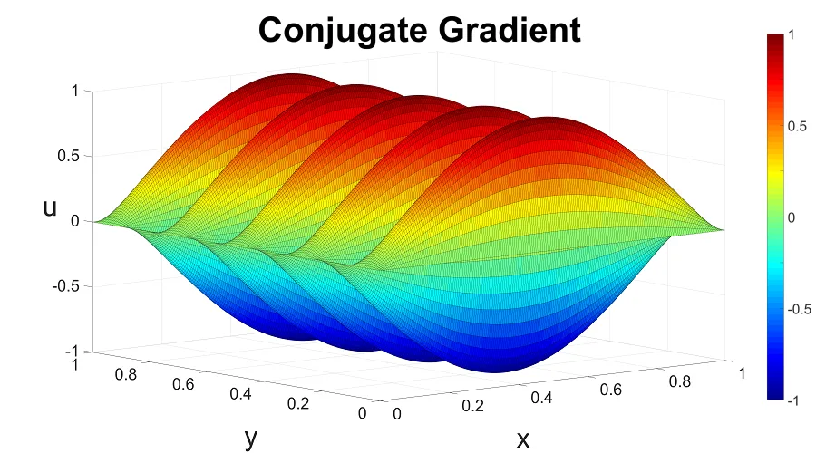
Let's go back to 2D Poisson's equation on a unit square domain, with homogeneous Dirichlet BC. Our RHS function is given by,

f(x, y)=(a2+b2)π2sin⁡(aπx)sin⁡(bπy),f(x,\,y) = (a^{2} + b^{2})\pi^{2}\sin(a\pi x)\sin(b\pi y),

and we choose a=1a = 1, b=9b = 9, and N=200N = 200 as before.

Stunningly, CG converges in 1 iteration! As far as iterative methods go, you can't do better than that.

CG converges in 1 iteration!

The question is how? The RHS function that I chose makes the Poisson's equation an eigenfunction problem. Even at the discrete level, the RHS vector f⃗\vec{f} happens to be an eigenvector of KK:

Kf⃗=λf⃗.K\vec{f} = \lambda\vec{f}.

As a result, in the first iteration,

α1 = f⃗Tf⃗f⃗TKf⃗ = 1λr⃗1 = f⃗−α1Kf⃗ = f⃗−1λ⋅λf⃗ = 0⃗.\begin{array}{l} \displaystyle\alpha_{1} \,=\, \frac{\vec{f}^{T}\vec{f}}{\vec{f}^{T}K\vec{f}} \,=\, \frac{1}{\lambda} \\ \displaystyle\vec{r}_{1} \,=\, \vec{f} - \alpha_{1}K\vec{f} \,=\, \vec{f} - \frac{1}{\lambda} \cdot \lambda\vec{f} \,=\, \vec{0}. \end{array}

Talk about luck (or well-planning)!

Notes

A big thanks goes to Dr. Ye, one of my teachers at Kentucky. He instilled my passion for numerical linear algebra and applications thereof. To learn additional iterative methods, I recommend reading his paper linked below.
You can find the code in its entirety here: Download from GitHub

References