Iterative Methods: Part 2

Last time, we looked at 2D Poisson's equation and discussed how to arrive at a matrix equation using the finite difference method. The matrix, which represents the discrete Laplace operator, is sparse, so we can use an iterative method to solve the equation efficiently.

Today, we will look at Jacobi, Gauss-Seidel, Successive Over-Relaxation (SOR), and Symmetric SOR (SSOR), and a couple of related techniques—red-black ordering and Chebyshev acceleration. In addition, we will analyze the convergence of each method for the Poisson's equation, both analytically and numerically.

2. Classical iterative methods

Recall that we placed $N$ interior points along each axis. Since we did not know the values of $u_{i,\,j} := u(x_{i},\,y_{j})$ at $N^{2}$ points, we had to solve $N^{2}$ equations.

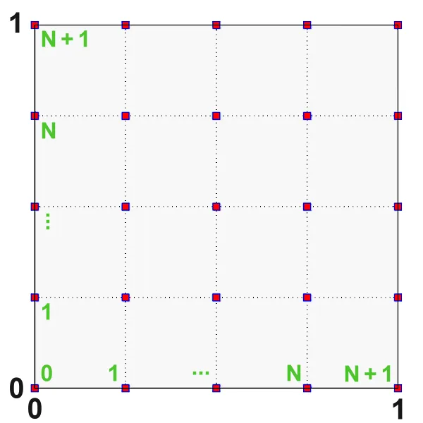
Each row in the equation $K\vec{u} = \vec{f}$ looked like,

where $h$ is the mesh size:

We also looked at the general equation $A\vec{x} = \vec{b}$, and discussed splitting the matrix into a sum of two matrices:

Note that $P$ is nonsingular. This let us define an iterative method based on fixed-point method. Given an initial guess $\vec{x}_{0}$, we can solve the following equation to find the next iterate $\vec{x}_{1}$, then $\vec{x}_{2}$, and so on:

Lastly, we defined the matrix,

and concluded that the iterative method converges from any initial guess, if and only if, the spectral radius $\rho(R)$ is less than 1.

Before we move on, let us define the rate of convergence:

The smaller the spectral radius of $R$, the higher the rate of convergence. We will see that, for each method, the spectral radius takes the form of $1 - x$ for some $x \in (0,\,1)$. Using Taylor expansion, we can write,

When $k$ is sufficiently large, we can interpret $1/r$ as the number of iterations further needed to reduce the error $||\vec{u}_{k} - \vec{u}||$ by a factor of $e$.

c. Jacobi

For Jacobi method, we split $A \in \mathbb{R}^{n \times n}$ as follows:

where,

Let's look at the fixed-point equation entry-wise:

Note that, for efficiency, we do not invert the matrix $P$ (i.e. use ** in Matlab) to solve the fixed-point equation. Instead, we consider the action of $P$ to deduce the action of $P^{-1}$. We can do so by writing the matrix equation entry-wise like we did above.

Since the diagonals are nonzero, we can divide both sides of the equation by $a_{ii}$. This is the action of $P^{-1}$ for Jacobi. We can now compute $x_{i}^{(k + 1)}$, the $i$-th entry of $\vec{x}_{k + 1}$:

Notice how we use information from the $k$-th iteration to determine the solution at the $(k + 1)$-th iteration. The diagram below shows which entries we would use to find the 2nd entry of $\vec{x}_{k + 1}$.

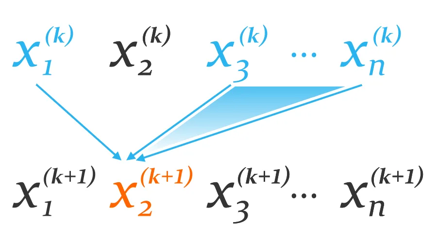
For Poisson's equation, the diagonals of $K$ are always 4, while the off-diagonals are either 0 or -1. Hence, Jacobi method simplifies to the following:

Jacobi, 2D Poisson's equation

$$\displaystyle\boxed{u_{i,\,j}^{(k + 1)} = \frac{1}{4}\left[u_{i-1,\,j}^{(k)} + u_{i+1,\,j}^{(k)} + u_{i,\,j-1}^{(k)} + u_{i,\,j+1}^{(k)} + h^{2}f_{ij}\right]}$$

As we can see below, it's easy to implement Jacobi method.

% Set initial guess u
u = [...];
 
% Set temporary variable
uNew = zeros(N + 2);
 
for k = 1 : numIterations
  % Natural ordering
  for j = 2 : (N + 1)
    for i = 2 : (N + 1)
      uNew(i, j) = 1/4 * (u(i - 1, j) + u(i + 1, j) + u(i, j - 1) + u(i, j + 1) + h^2*f(i, j));
    end
  end
 
  % Update iterate
  u = uNew;
end

Finally, let's analyze the convergence of Jacobi method for Poisson's equation. We use the fact that the eigenvalues of $K$ are given by,

Convergence of Jacobi, 2D Poisson's equation

$$\displaystyle\boxed{\rho(R) = \cos(h\pi) \approx 1 - \frac{1}{2}h^{2}\pi^{2}}$$

Proof.

First, let's find the eigenvalues of $R = P^{-1}Q$. Fortunately, we can write $P = 4I$ and $P^{-1} = \frac{1}{4}I$. Therefore,

Hence, we can find the eigenvalues of $R$ from those of $K$:

The spectral radius $\rho(R)$, which is the largest eigenvalue of $R$ in magnitude, occurs when $i$ and $j$ are both equal to 1 (or $N$ by symmetry). We use Taylor expansion to conclude that,

■

Since $\rho(R) \approx 1 - \frac{1}{2}h^{2}\pi^{2} < 1$, Jacobi converges for Poisson's equation. Unfortunately, as we increase $N$ to refine the domain, the spectral radius approaches 1 quadratically. After some time, in order for Jacobi to reduce the error by $e$, we need to perform

additional iterations. Can we do better?

d. Gauss-Seidel

This time, we split $A$ as follows:

where $D,\,L,\,U$ are defined in the exact manner as in Jacobi.

Let's analyze the action of $P^{-1}$:

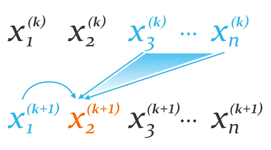
Now comes the clever idea. By the time we compute $x_{i}^{(k + 1)}$, we will have computed the previous entries $x_{0}^{(k + 1)},\,\cdots,\,x_{i - 1}^{(k + 1)}$. These values are more accurate than those from the previous iteration $x_{0}^{(k)},\,\cdots,\,x_{i - 1}^{(k)}$, so we use them to compute $x_{i}^{(k + 1)}$:

Finally, we divide both sides of the equation by $a_{ii}\,(\neq 0)$:

We can visualize the similarities and dissimilarities between Jacobi and Gauss-Seidel with the diagram below.

Gauss-Seidel, 2D Poisson's equation

$$\displaystyle\boxed{u_{i,\,j}^{(k + 1)} = \frac{1}{4}\left[u_{i-1,\,j}^{(k + 1)} + u_{i+1,\,j}^{(k)} + u_{i,\,j-1}^{(k + 1)} + u_{i,\,j+1}^{(k)} + h^{2}f_{ij}\right]}$$

Convergence of Gauss-Seidel, 2D Poisson's equation

$$\boxed{\rho(R) = \cos^{2}(h\pi) \approx 1 - h^{2}\pi^{2}}$$

Proof.

We use the fact that, $\lambda \neq 0$ is an eigenvalue of $R_{J}$, if and only if, $\lambda^{2}$ is an eigenvalue of $R_{GS}$. This holds when the matrix $A$ is consistently ordered (I won't define this here).

For now, assume that $K$ is consistently ordered. Then,

■

The number of iterations further needed to reduce the error by $e$ is,

which is half of that of Jacobi.

Let's resolve the caveat. For our problem, $K$ can be consistently ordered if we traverse the points in a checkerboard fashion, also known as red-black ordering.

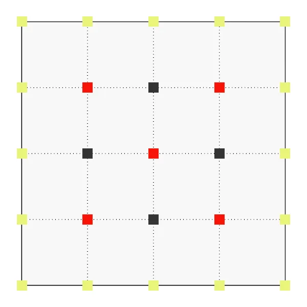
The red points are updated first using the previous iterate, then the black points using the updated red points. Note that Gauss-Seidel does converge if we traverse the points in the natural order. However, we will not achieve optimal convergence. This will also be the case when we look at Successive Over-Relaxation.

We summarize Gauss-Seidel with a pseudocode below. Notice that we no longer need the temporary variable uNew.

% Set initial guess u
u = [...];
 
for k = 1 : numIterations
  % Red points
  for j = 2 : (N + 1)
    for i = 2 : (N + 1)
      if (mod(i + j, 2) == 0)
        u(i, j) = 1/4 * (u(i - 1, j) + u(i + 1, j) + u(i, j - 1) + u(i, j + 1) + h^2*f(i, j));
      end
    end
  end
 
  % Black points
  for j = 2 : (N + 1)
    for i = 2 : (N + 1)
      if (mod(i + j, 2) == 1)
        u(i, j) = 1/4 * (u(i - 1, j) + u(i + 1, j) + u(i, j - 1) + u(i, j + 1) + h^2*f(i, j));
      end
    end
  end
end

e. Successive Over-Relaxation

Gauss-Seidel takes the current iterate $\vec{x}_{k}$ to the next $\vec{x}_{k + 1}$ better than Jacobi. Why not take a step further in the direction that Gauss-Seidel points us to?

This is the motivation behind Successive Over-Relaxation (SOR). We take a weighted average of the current iterate $\vec{x}_{k}$ and the next iterate $\vec{x}_{k + 1,\,GS}$ that Gauss-Seidel gives, to arrive at the final result $\vec{x}_{k + 1}$.

Entry-wise, this means the following:

Note that, if $\omega = 1$, we get Gauss-Seidel back.

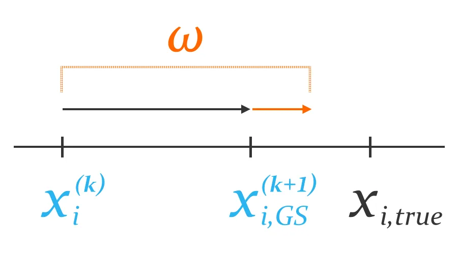
The weight $\omega$ cannot be arbitrary. We can show that, if SOR converges, then $\omega \in (0,\,2)$. In other words, we would never set $\omega \leq 0$ or $\omega \geq 2$. We also have a simple, sufficient condition for convergence:

Convergence of SOR

If the matrix $A$ is positive definite, that is,

$$\vec{x}^{T}A\vec{x} > 0,\,\,\,\text{for all}\,\,\vec{x} \neq \vec{0},$$

then SOR converges for any $\omega \in (0,\,2)$.

For our problem, we know that $K$ is positive definite because all of its eigenvalues are positive. While we can choose any $\omega \in (0,\,2)$ for convergence, the optimal value that leads to a fixed tolerance the quickest is given by,

Again, we want a consistently ordered $K$ for optimal convergence, so we will traverse the points using red-black ordering instead of natural ordering.

We summarize SOR for Poisson's equation below:

SOR, 2D Poisson's equation

$$\boxed{\left\{\begin{array}{l} \displaystyle\omega = \frac{2}{1 + \sin(h\pi)} \\ \displaystyle u_{i,\,j}^{(k + 1)} = (1 - \omega)\,u_{i,\,j}^{(k)} + \frac{\omega}{4}\left[u_{i-1,\,j}^{(k + 1)} + u_{i+1,\,j}^{(k)} + u_{i,\,j-1}^{(k + 1)} + u_{i,\,j+1}^{(k)} + h^{2}f_{ij}\right] \end{array}\right.}$$

Convergence of SOR, 2D Poisson's equation

$$\displaystyle\boxed{\rho(R) = \frac{\cos^{2}(h\pi)}{(1 + \sin(h\pi))^{2}} \approx 1 - 2h\pi}$$

This time, as we refine the domain, the spectral radius approaches 1 only linearly. The number of iterations further needed to reduce the error by $e$ is,

about $N$ times less than Jacobi and Gauss-Seidel!

f. Symmetric SOR

In Symmetric SOR (SSOR), we take a half-step of SOR in the natural order, then take another half-step of SOR in the reverse order. John Sheldon, who published SSOR in 1955, had gotten inspiration from "a computer which has magnetic tapes which read 'backward' as well as 'forward.'"

SSOR alone does not produce a solution much different from that from SOR. In fact, for every iteration of SSOR, we incur 2 iterations of SOR. However, when we consider an auxiliary problem known as Chebyshev acceleration, SSOR can reach convergence an order of magnitude faster. I won't explain why Chebyshev acceleration works, but will provide the pseudocode and implement it in our program.

% Set temporary variables
rho = 1 - pi/(2*N);
mu0 = 1;
mu1 = rho;
 
% Set initial guess u0
u0 = [...];
 
% Perform 1 iteration of SSOR
u1 = [...];
 
% Perform the remaining iterations
for k = 2 : numIterations
  mu = 1 / (2/(rho*mu1) - 1/mu0);
 
  % Perform 1 iteration of SSOR
  u = [...];
 
  % Apply Chebyshev acceleration
  u = 2*mu/(rho*mu1) * u - mu/mu0 * u0;
 
  % Update temporary variables
  mu0 = mu1;
  mu1 = mu;
  u0  = u1;
  u1  = u;
end

Since SSOR uses SOR, we need to select the weight $\omega$. For 2D Poisson's equation, David Young recommends

which results in the following spectral radius:

The rate of convergence does not seem to be different from that for SOR. However, with Chebyshev acceleration, we can multiply the error by $\mu_{k}$ (denoted mu in the code) at the $k$-th iteration. We have an upper bound for $\mu_{k}$:

3. Example

Recall that our model problem uses the RHS function,

We choose $a = 1$ and $b = 9$ (the number of ridges in $x$ and $y$-directions) and $N = 200$. For each method, we graph the approximate solution after 100 iterations, and plot the error $||\vec{u}_{k} - \vec{u}||_{2}$ every 50 iterations. We will stop the method once $k$ reaches 500.

To compute the error $||\vec{u}_{k} - \vec{u}||_{2}$ at the $k$-th iteration, we need to know the solution $\vec{u}$. We can approximate it by considering the SSOR solution at 1000th iteration to be the exact solution, i.e. $\vec{u} \,\approx\, \vec{u}_{1000}$.

a. Results

After 100 iterations, we get the following solutions:

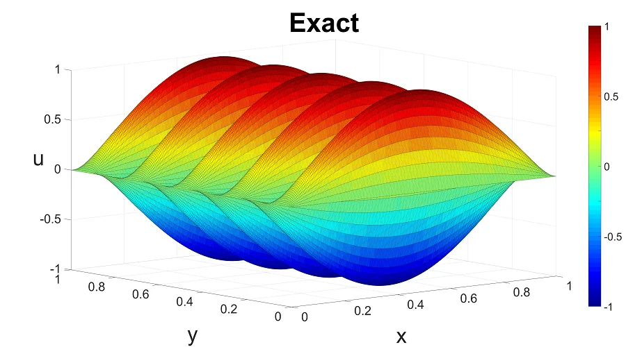
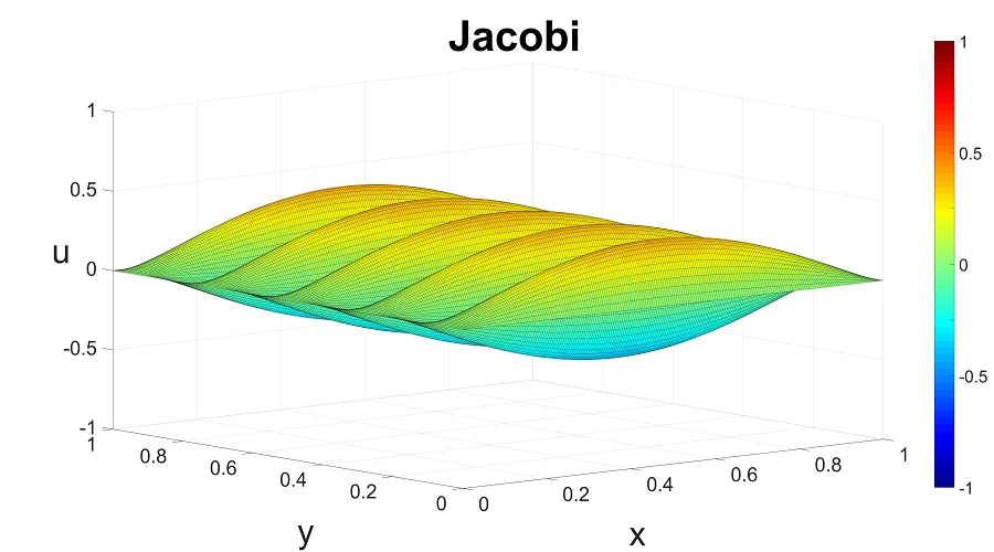
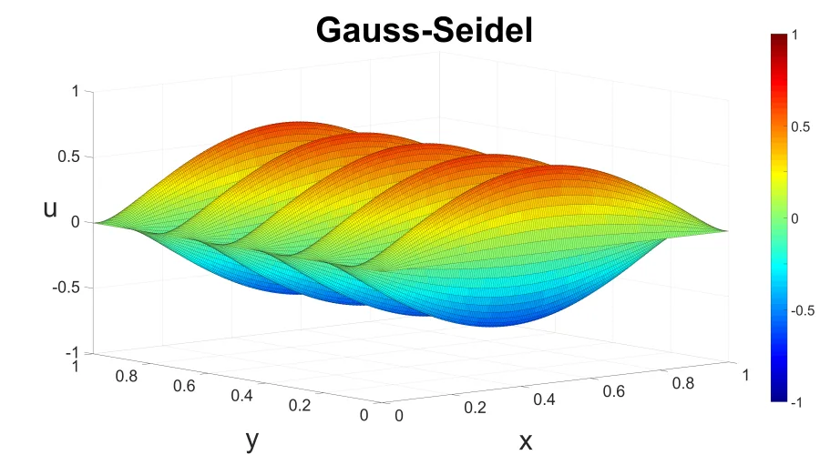
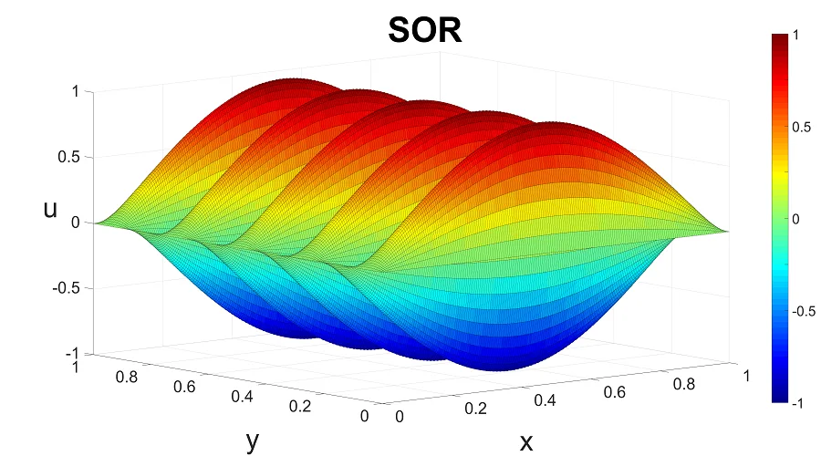
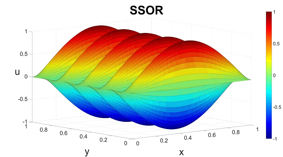
We can see that Gauss-Seidel is twice better than Jacobi. The amplitude of the Jacobi solution is about 0.40, while that of Gauss-Seidel is 0.64. The $l^{2}$-error, $||\vec{u}_{100} - \vec{u}||_{2}$, is about 61.0 for Jacobi, and 37.0 for Gauss-Seidel. SOR and SSOR produce even better result: an amplitude close to 1 and an $l^{2}$-error of about 3.3 and 0.0, respectively.

Next, let's check the behavior of the $l^{2}$-error $||\vec{u}_{k} - \vec{u}||_{2}$. We take the base-10 logarithm of the error to focus on its magnitude.

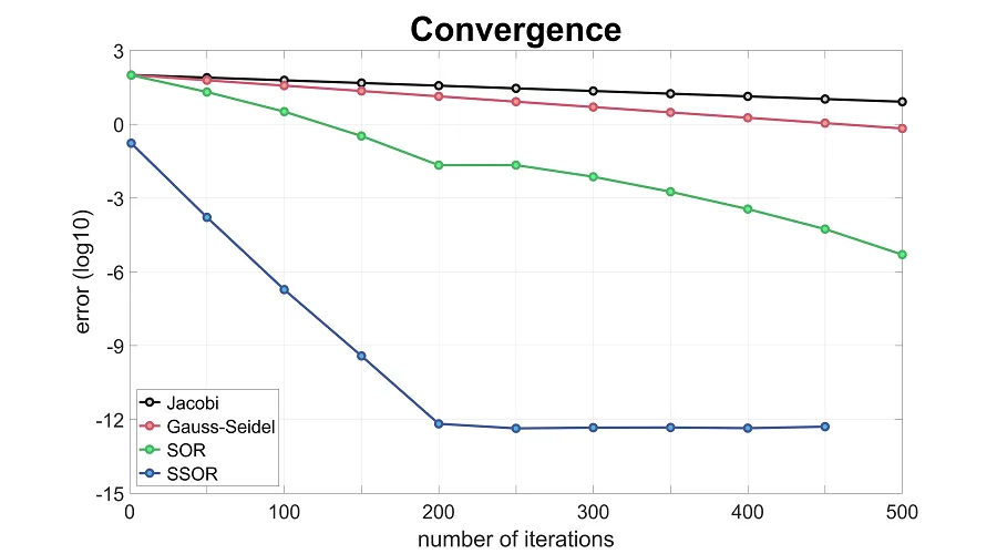
From the slopes, we see that the error for Gauss-Seidel decreases twice as fast as that for Jacobi. However, even after 500 iterations, the errors remain large. In comparison, the error for SOR almost reaches $10^{-6}$ (okay in practice) after 500 iterations, while that for SSOR reaches $10^{-12}$ (true convergence) after 200 iterations! We may equate this to about 400 SOR iterations.

b. What if

I mentioned that, for optimal convergence, we want to follow red-black ordering for Gauss-Seidel and SOR, and to add Chebyshev acceleration to SSOR. Let's see what happens if we follow natural ordering for Gauss-Seidel and SOR, and perform SSOR without Chebyshev acceleration.

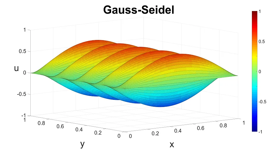
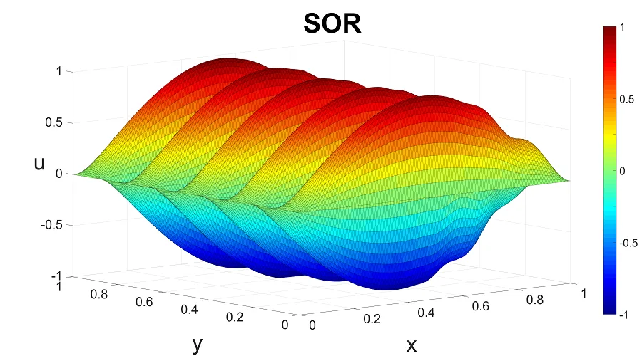
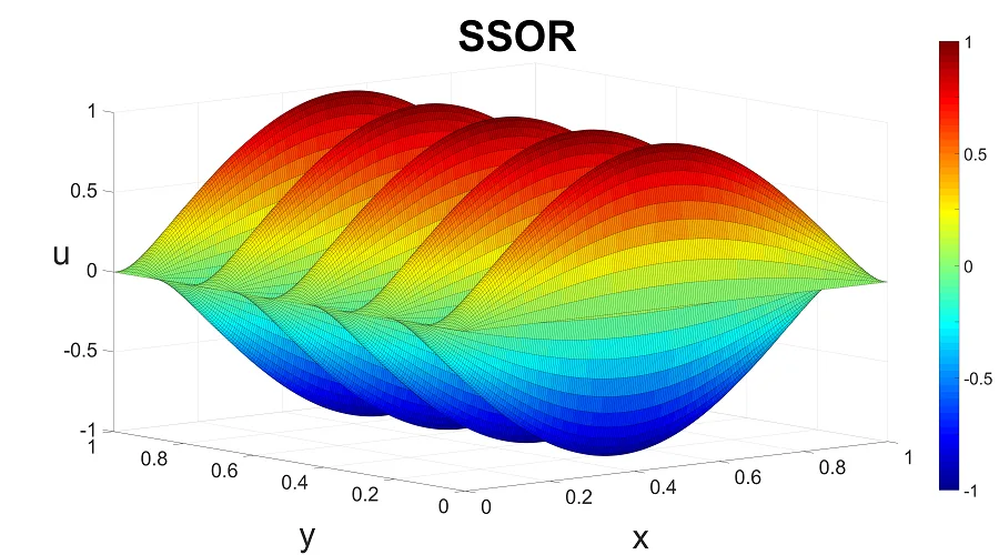
After 100 iterations, the SOR solution is perhaps graphically the most different. We see a funny oscillation on the right part of the domain, perhaps because we traversed the points from left to right. (I would have suspected the left side to be less accurate, and wonder if I reversed the graph by mistake.) The oscillation goes away as we increase the number of iterations, but is undesirable in the first place.

If we look at the convergence plot, we can understand even better why we should not use natural ordering for SOR or omit Chebyshev acceleration for SSOR.

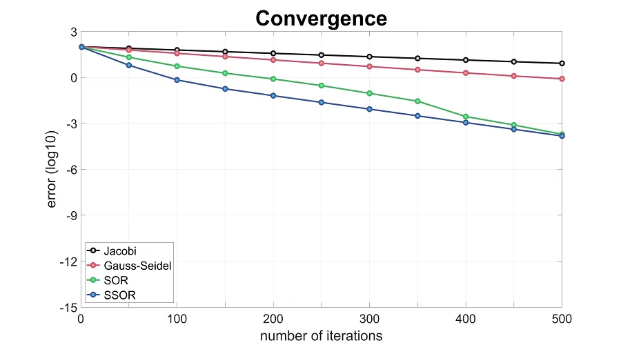
This time, the error for SOR only reaches $10^{-4}$ after 500 iterations. SSOR converges faster than SOR initially, but the error also reaches $10^{-4}$ after 500 iterations. This is especially frustrating, since for each SSOR iteration, we performed 2 SOR iterations. Note that the choice of $\omega$ is the same as before:

Notes

In short, use SSOR with Chebyshev acceleration. In addition to solving equations, SSOR makes a great preconditioner. Next time, we will look at Conjugate Gradient method, which is useful when the matrix is symmetric, positive definite (SPD).

You can find the code in its entirety here: Download from GitHub

References

• James Demmel, Applied Numerical Linear Algebra (1997), 279-299.
• Isaac Lee, lecture notes (2011).
• John Sheldon, On the Numerical Solution of Elliptic Difference Equations, Mathematical Tables and Other Aids to Computation 9 (1955), 101-112.
• Qiang Ye, lecture notes (2009).