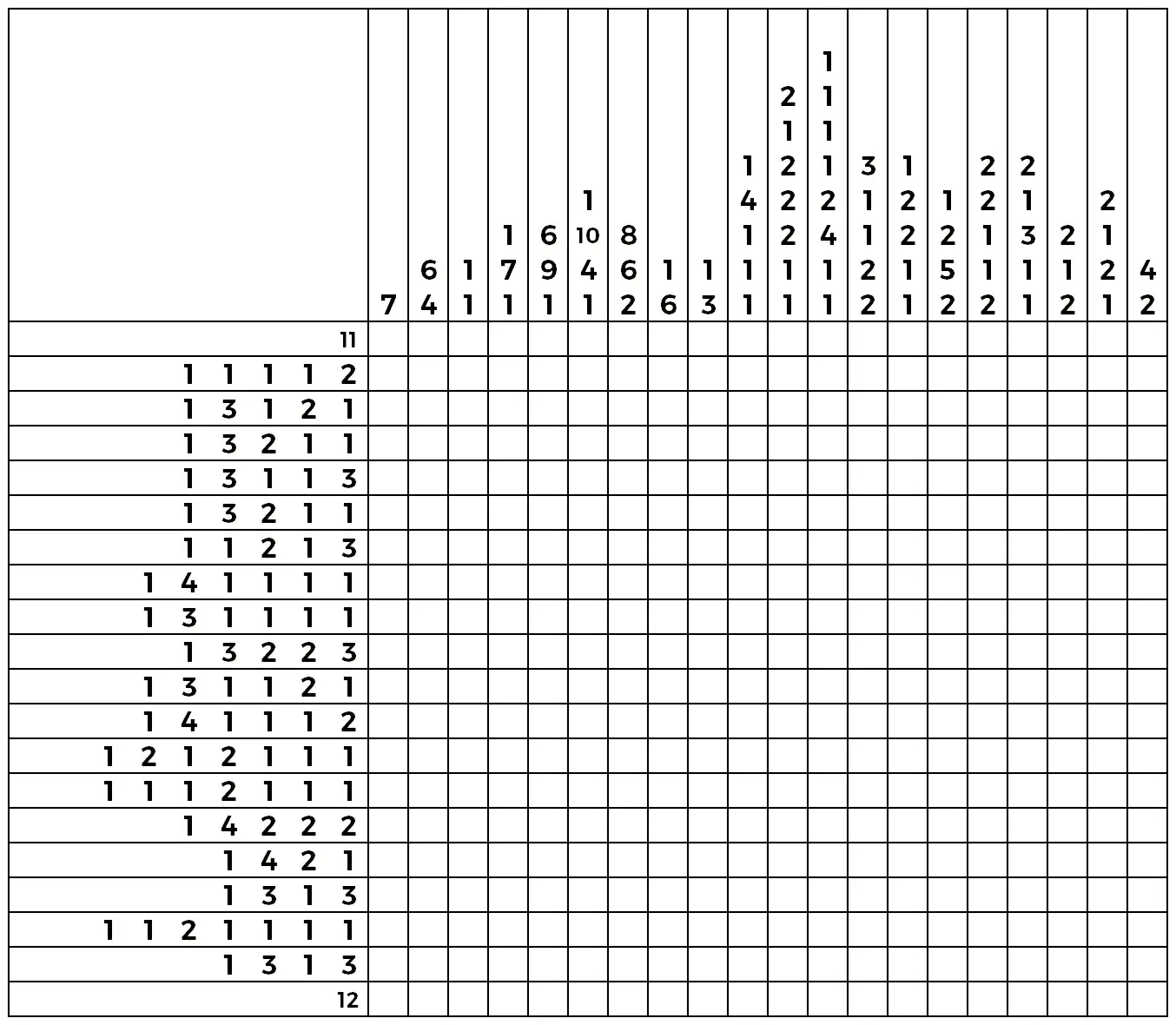
Solving Nonograms with Compressive Sensing: Part 3

We know how to represent the solution of a nonogram as a sparse vector $\vec{x} \in \{0,\,1\}^{N}$. Let us now design the constraints; they will be linear equations and linear inequalities that the entries of $\vec{x}$ must satisfy according to the nonogram. The only information that the nonogram provides are the row and column sequences, so we want to make the most of it. Afterwards, we obtain the sparse vector $\vec{x}$ by minimizing its 1-norm under these constraints. I will discuss the code and the results in the next and final post.

4. Designing constraints

Recall that our basis vectors lie along the row direction. As a result, it is hard to use row basis vectors to ensure that we satisfy the column sequences. We can only require the column sums to be satisfied.

We can do a lot more with the row sequences. We will have one set of linear equality constraints that counts how many times each block size appears in a row sequence. Clearly, this is better than asking the row sums to be satisfied. We will also have two sets of linear inequality constraints that enforce the rules of the nonogram.

The $l^{1}$-minimization problem takes the form,

$$\boxed{\begin{array}{rl} \displaystyle \min_{\vec{x} \,\in\, \{0,\,1\}^{N}} & ||\vec{x}||_{1} \\ \text{subject to} & A\vec{x} = \vec{b} \\ & B\vec{x} \leq \vec{c}. \end{array}}$$

for some matrices $A \in \mathbb{R}^{M_{1} \times N}$, $B \in \mathbb{R}^{M_{2} \times N}$ and for some vectors $\vec{b} \in \mathbb{R}^{M_{1}}$, $\vec{c} \in \mathbb{R}^{M_{2}}$. We will determine how large $M_{1}$ and $M_{2}$ are at the end.

Note that, by definition, the 1-norm of a vector is the sum of its entries in magnitude:

$$\displaystyle ||\vec{x}||_{1} \,=\, \sum_{i\,=\,1}^{N}\,\,|x_{i}|.$$

The entries $x_{i}$ (these are the basis vectors $e_{ikj}$ in their natural order) are either 0 or 1, and both of these values are nonnegative. Therefore, we can write instead,

$$\displaystyle\boxed{||\vec{x}||_{1} \,=\, \sum_{i\,=\,1}^{N}\,\,x_{i}}.$$

Matlab needs us to write the objective function as a linear combination of the solution vector's entries. The equation above shows that $||\vec{x}||_{1}$ is a linear combination of the entries of $\vec{x}$, with coefficients of 1.

a. Sparsity level

Unlike in most optimization problems, we know the minimum value that our objective function $||\vec{x}||_{1}$ should reach. It is equal to the sparsity level $s$. (Recall that $s$ equals how many numbers appear in the row sequences, so we know its value.)

We pass this information to our solver as a linear equation:

$$\displaystyle\boxed{\sum_{i\,=\,1}^{N}\,\,x_{i} \,=\, s}.$$

We can write this as a matrix equation $A_{1}\vec{x} = \vec{b}_{1}$. $A_{1}$ is a $1 \times N$ matrix whose entries are all 1, and $\vec{b}_{1}$ is a vector with just one entry, $s$.

b. Column sums

Consider the $J$-th column, where $J$ is a number between 1 and $n$. From the column sequence $(b_{1},\,\cdots,\,b_{p})$, we can find the column sum $r = b_{1} + \cdots + b_{p}$. Recall that the column sum tells us how many cells on the $J$-th column must be shaded. There are $N$ basis vectors, and we want exactly $r$ among them to pass the $J$-th column.

Well, which basis vectors can pass the $J$-th column? To answer this question, we consider one of the rows. We can list the basis vectors that pass the $J$-th column in the following manner:

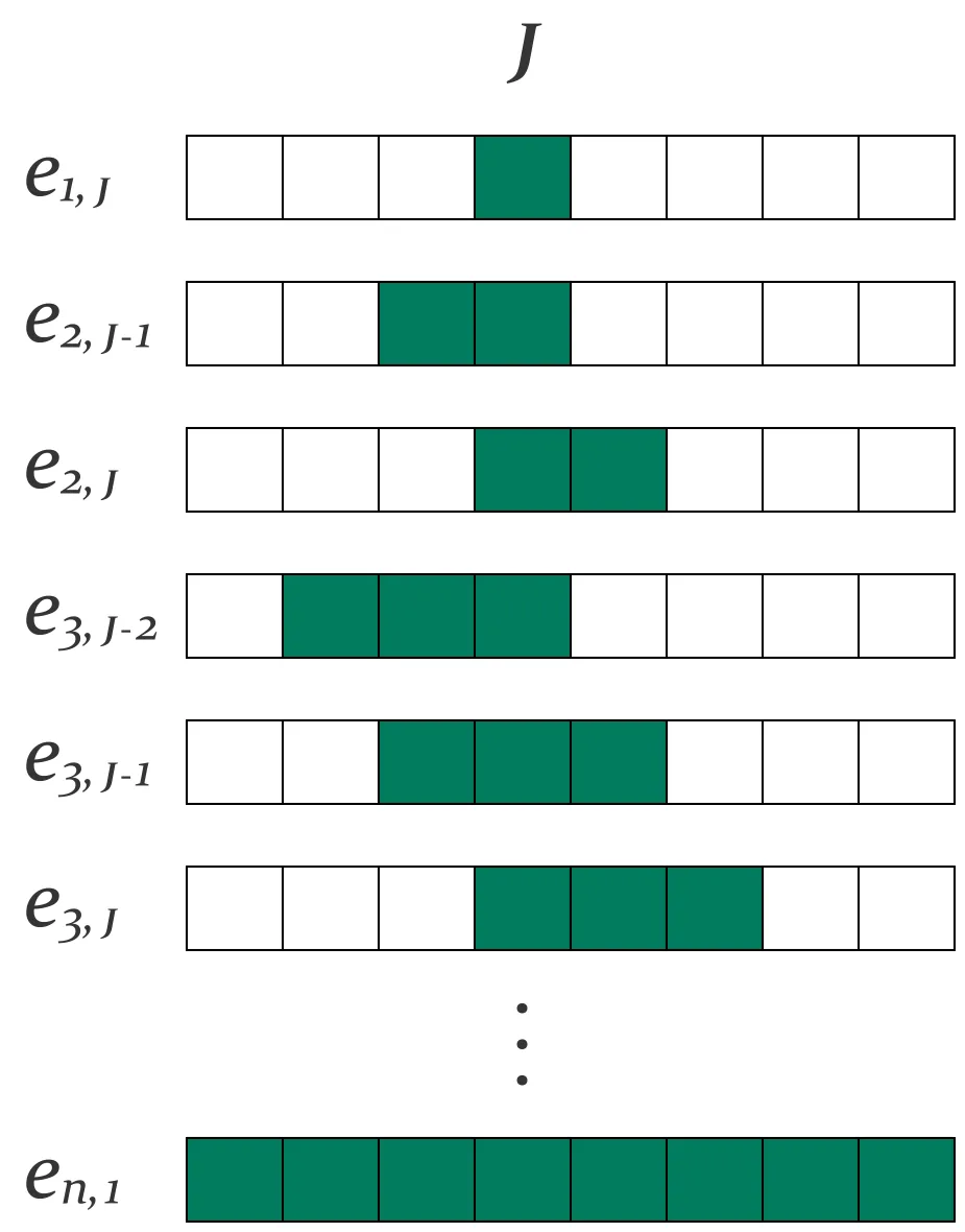
Which basis vectors $e_{kj}$ have we considered above? Clearly, $k$ ranges between 1 and $n$, i.e. for each block size, there exists a basis vector that passes the $J$-th column.

What about $j$, the starting column index? The lowest that $j$ can be and still allow the basis vector to pass the $J$-th column certainly depends on the block size $k$. From our list of basis vectors above, we conclude $(J - k + 1)$. It is possible that this number is less than 1, which would not make sense. We stop this from happening by selecting the larger between $(J - k + 1)$ and 1.

The highest that $j$ can be is $(n - k + 1)$. We saw this number when we designed the basis vectors last time. If this number is greater than $J$, then the basis vector would start somewhere after the $J$-th column instead of passing it. Therefore, we consider the smaller between $(n - k + 1)$ and $J$.

In summary, the basis vectors $e_{kj}$ that pass the $J$-th column are those whose indices satisfy,

$$\begin{array}{l} k = 1,\,\cdots,\,n \\ j = j_{lo},\,\cdots,\,j_{hi}, \end{array}$$

where,

$$\begin{array}{l} j_{lo} = \max\bigl\{J - k + 1,\,\,1\bigr\} \\ j_{hi} = \min\bigl\{n - k + 1,\,\,J\bigr\}. \end{array}$$

The $J$-th column sum is satisfied if we require that

$$\displaystyle\boxed{\sum_{i\,=\,1}^{m}\,\,\sum_{k\,=\,1}^{n}\,\sum_{j\,=\,j_{lo}}^{j_{hi}}\,e_{ikj} \,=\, r}.$$

We use the natural order of the basis vectors to arrive at a linear system $A_{2}\vec{x} = \vec{b}_{2}$, where $A_{2}$ is a $n \times N$ matrix.

For the stylish lambda,

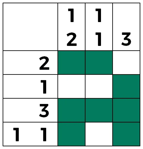
we have $A_{2} \in \mathbb{R}^{3 \times 24}$ and $\vec{b}_{2} \in \mathbb{R}^{3}$. Their entries are given by,

$$A_{2} = \left[\begin{array}{cccccc | cccccc | cccccc | cccccc} 1 & 0 & 0 & 1 & 0 & 1 & 1 & 0 & 0 & 1 & 0 & 1 & 1 & 0 & 0 & 1 & 0 & 1 & 1 & 0 & 0 & 1 & 0 & 1 \\ 0 & 1 & 0 & 1 & 1 & 1 & 0 & 1 & 0 & 1 & 1 & 1 & 0 & 1 & 0 & 1 & 1 & 1 & 0 & 1 & 0 & 1 & 1 & 1 \\ 0 & 0 & 1 & 0 & 1 & 1 & 0 & 0 & 1 & 0 & 1 & 1 & 0 & 0 & 1 & 0 & 1 & 1 & 0 & 0 & 1 & 0 & 1 & 1 \end{array}\right]$$ $$\vec{b}_{2} = \bigl[\,\,3\,\, \,\, \,\,2\,\, \,\, \,\,3\,\,\bigr]^{T}.$$

The 1's on the first row of $A_{2}$ correspond to all basis vectors that pass the first column, the 1's on the second row the second column, and the 1's on the third row the third column. The entries of $\vec{b}_{2}$ are the column sums.

c. Block counts

Let us now consider the row sequences. Consider the $I$-th row, where $I$ is a number between 1 and $m$. From the row sequence, we can determine $t_{K}$, how many times blocks of size $K$ should appear on the $I$-th row.

We write the following equations for the $I$-th row:

$$\displaystyle\boxed{\sum_{j\,=\,1}^{j_{hi}}\,e_{IKj} \,=\, t_{K},\,\,\,\text{for}\,\,K = 1,\,\cdots,\,n},$$

where,

$$j_{hi} = n - K+ 1.$$

These equations are true, since the left-hand side counts how many basis vectors of size $K$ we use, and this must equal how many times $K$ appears in the row sequence. We use the natural order and arrive at $A_{3}\vec{x} = \vec{b}_{3}$, where $A_{3}$ is a $mn \times N$ matrix.

For the stylish lambda, we find that $A_{3} \in \mathbb{R}^{12 \times 24}$ and $\vec{b}_{3} \in \mathbb{R}^{12}$. Their entries are shown below (see if you can make sense of them):

$$A_{3} = \left[\begin{array}{cccccc | cccccc | cccccc | cccccc} 1 & 1 & 1 & 0 & 0 & 0 & 0 & 0 & 0 & 0 & 0 & 0 & 0 & 0 & 0 & 0 & 0 & 0 & 0 & 0 & 0 & 0 & 0 & 0 \\ 0 & 0 & 0 & 1 & 1 & 0 & 0 & 0 & 0 & 0 & 0 & 0 & 0 & 0 & 0 & 0 & 0 & 0 & 0 & 0 & 0 & 0 & 0 & 0 \\ 0 & 0 & 0 & 0 & 0 & 1 & 0 & 0 & 0 & 0 & 0 & 0 & 0 & 0 & 0 & 0 & 0 & 0 & 0 & 0 & 0 & 0 & 0 & 0 \\ \hline 0 & 0 & 0 & 0 & 0 & 0 & 1 & 1 & 1 & 0 & 0 & 0 & 0 & 0 & 0 & 0 & 0 & 0 & 0 & 0 & 0 & 0 & 0 & 0 \\ 0 & 0 & 0 & 0 & 0 & 0 & 0 & 0 & 0 & 1 & 1 & 0 & 0 & 0 & 0 & 0 & 0 & 0 & 0 & 0 & 0 & 0 & 0 & 0 \\ 0 & 0 & 0 & 0 & 0 & 0 & 0 & 0 & 0 & 0 & 0 & 1 & 0 & 0 & 0 & 0 & 0 & 0 & 0 & 0 & 0 & 0 & 0 & 0 \\ \hline 0 & 0 & 0 & 0 & 0 & 0 & 0 & 0 & 0 & 0 & 0 & 0 & 1 & 1 & 1 & 0 & 0 & 0 & 0 & 0 & 0 & 0 & 0 & 0 \\ 0 & 0 & 0 & 0 & 0 & 0 & 0 & 0 & 0 & 0 & 0 & 0 & 0 & 0 & 0 & 1 & 1 & 0 & 0 & 0 & 0 & 0 & 0 & 0 \\ 0 & 0 & 0 & 0 & 0 & 0 & 0 & 0 & 0 & 0 & 0 & 0 & 0 & 0 & 0 & 0 & 0 & 1 & 0 & 0 & 0 & 0 & 0 & 0 \\ \hline 0 & 0 & 0 & 0 & 0 & 0 & 0 & 0 & 0 & 0 & 0 & 0 & 0 & 0 & 0 & 0 & 0 & 0 & 1 & 1 & 1 & 0 & 0 & 0 \\ 0 & 0 & 0 & 0 & 0 & 0 & 0 & 0 & 0 & 0 & 0 & 0 & 0 & 0 & 0 & 0 & 0 & 0 & 0 & 0 & 0 & 1 & 1 & 0 \\ 0 & 0 & 0 & 0 & 0 & 0 & 0 & 0 & 0 & 0 & 0 & 0 & 0 & 0 & 0 & 0 & 0 & 0 & 0 & 0 & 0 & 0 & 0 & 1 \end{array}\right]$$ $$\vec{b}_{3} = \bigl[\,\,0\,\, \,\, \,\,1\,\, \,\, \,\,0\,\, \,|\, \,\,1\,\, \,\, \,\,0\,\, \,\, \,\,0\,\, \,|\, \,\,0\,\, \,\, \,\,0\,\, \,\, \,\,1\,\, \,|\, \,\,2\,\, \,\, \,\,0\,\, \,\, \,\,0\,\, \bigr]^{T}.$$

d. Nonogram rules! (part 1)

One of the rules of nonogram is that we must have at least one empty cell between two consecutive blocks of shaded cells. Necessarily, certain basis vectors $e_{kj}$ on the same row cannot appear together. We cannot have $e_{11} = 1$ and $e_{12} = 1$, for example. Since $e_{kj}$ take on binary values, we can require that $e_{11} + e_{12} \leq 1$ to force one of the two variables to be zero.

The stylish lambda, which has 3 columns, lends these inequalities for each row:

$$\begin{array}{l} e_{11} + e_{12} \leq 1 \text{\hspace{1cm}} e_{11} + e_{21} \leq 1 \text{\hspace{1cm}} e_{11} + e_{22} \leq 1 \text{\hspace{1cm}} e_{11} + e_{31} \leq 1 \\ e_{12} + e_{13} \leq 1 \text{\hspace{1cm}} e_{12} + e_{21} \leq 1 \text{\hspace{1cm}} e_{12} + e_{22} \leq 1 \text{\hspace{1cm}} e_{12} + e_{31} \leq 1 \\ e_{13} + e_{21} \leq 1 \text{\hspace{1cm}} e_{13} + e_{22} \leq 1 \text{\hspace{1cm}} e_{13} + e_{31} \leq 1 \\ e_{21} + e_{22} \leq 1 \text{\hspace{1cm}} e_{21} + e_{31} \leq 1 \\ e_{22} + e_{31} \leq 1. \end{array}$$

Can you see a problem here? There are a total of 56 inequalities but only 24 unknown variables! We would be liars to call our approach compressive sensing when we make these many measurements. In general, the number of such inequalities is,

$$\displaystyle m \times \frac{1}{12}\bigl(n^{4} + 4n^{3} - n^{2} - 4n\bigr) \approx \frac{mn^{4}}{12}.$$

We arrive at a new insight by considering the following picture:

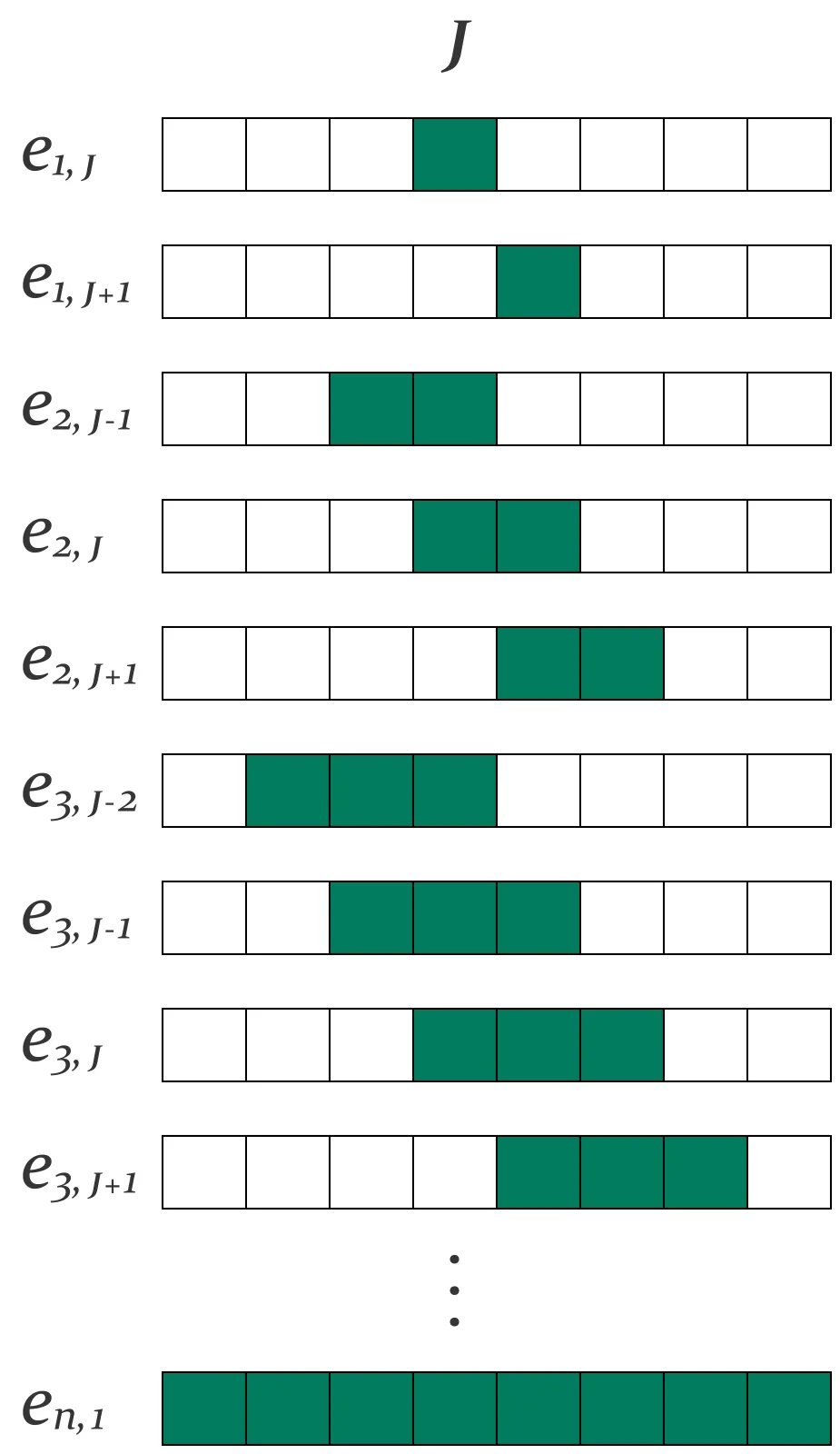
The picture looks similar to the one from Section 4b, where we considered all basis vectors that pass the $J$-th column. The only difference is that we added basis vectors that start at the $(J + 1)$-th column. We call these basis vectors mutually exclusive, because no pair among them should occur together. Check it!

For each $J$, we can ensure that the basis vectors are mutually exclusive with a linear inequality:

$$\displaystyle\boxed{\sum_{k\,=\,1}^{n}\,\sum_{j\,=\,j_{lo}}^{j_{hi}}\,e_{Ikj} \,\leq\, 1}.$$

The bounds of $j$ are given by,

$$\begin{array}{l} j_{lo} = \max\,\bigl\{J - k + 1,\,\,1\bigr\} \\ j_{hi} = \min\,\bigl\{n - k + 1,\,\,J + 1\bigr\}. \end{array}$$

We have such inequalities for each row, for a total of $mn$ constraints. We can use the natural order to write $B_{1}\vec{x} \leq \vec{c}_{1}$, where $B_{1}$ is a $mn \times N$ matrix. We are truly lucky that our solution vector takes binary values. How else could we combine (compress, heh) $mn^{4}/12$ amount of information into just $mn$?!

For the stylish lambda, $B_{1} \in \mathbb{R}^{12 \times 24}$ and $\vec{c}_{1} \in \mathbb{R}^{12}$ are as follows:

$$B_{1} = \left[\begin{array}{cccccc | cccccc | cccccc | cccccc} 1 & 1 & 0 & 1 & 1 & 1 & 0 & 0 & 0 & 0 & 0 & 0 & 0 & 0 & 0 & 0 & 0 & 0 & 0 & 0 & 0 & 0 & 0 & 0 \\ 0 & 1 & 1 & 1 & 1 & 1 & 0 & 0 & 0 & 0 & 0 & 0 & 0 & 0 & 0 & 0 & 0 & 0 & 0 & 0 & 0 & 0 & 0 & 0 \\ 0 & 0 & 1 & 0 & 1 & 1 & 0 & 0 & 0 & 0 & 0 & 0 & 0 & 0 & 0 & 0 & 0 & 0 & 0 & 0 & 0 & 0 & 0 & 0 \\ \hline 0 & 0 & 0 & 0 & 0 & 0 & 1 & 1 & 0 & 1 & 1 & 1 & 0 & 0 & 0 & 0 & 0 & 0 & 0 & 0 & 0 & 0 & 0 & 0 \\ 0 & 0 & 0 & 0 & 0 & 0 & 0 & 1 & 1 & 1 & 1 & 1 & 0 & 0 & 0 & 0 & 0 & 0 & 0 & 0 & 0 & 0 & 0 & 0 \\ 0 & 0 & 0 & 0 & 0 & 0 & 0 & 0 & 1 & 0 & 1 & 1 & 0 & 0 & 0 & 0 & 0 & 0 & 0 & 0 & 0 & 0 & 0 & 0 \\ \hline 0 & 0 & 0 & 0 & 0 & 0 & 0 & 0 & 0 & 0 & 0 & 0 & 1 & 1 & 0 & 1 & 1 & 1 & 0 & 0 & 0 & 0 & 0 & 0 \\ 0 & 0 & 0 & 0 & 0 & 0 & 0 & 0 & 0 & 0 & 0 & 0 & 0 & 1 & 1 & 1 & 1 & 1 & 0 & 0 & 0 & 0 & 0 & 0 \\ 0 & 0 & 0 & 0 & 0 & 0 & 0 & 0 & 0 & 0 & 0 & 0 & 0 & 0 & 1 & 0 & 1 & 1 & 0 & 0 & 0 & 0 & 0 & 0 \\ \hline 0 & 0 & 0 & 0 & 0 & 0 & 0 & 0 & 0 & 0 & 0 & 0 & 0 & 0 & 0 & 0 & 0 & 0 & 1 & 1 & 0 & 1 & 1 & 1 \\ 0 & 0 & 0 & 0 & 0 & 0 & 0 & 0 & 0 & 0 & 0 & 0 & 0 & 0 & 0 & 0 & 0 & 0 & 0 & 1 & 1 & 1 & 1 & 1 \\ 0 & 0 & 0 & 0 & 0 & 0 & 0 & 0 & 0 & 0 & 0 & 0 & 0 & 0 & 0 & 0 & 0 & 0 & 0 & 0 & 1 & 0 & 1 & 1 \end{array}\right]$$ $$\vec{c}_{1} = \bigl[\,\,1\,\, \,\, \,\,1\,\, \,\, \,\,1\,\, \,|\, \,\,1\,\, \,\, \,\,1\,\, \,\, \,\,1\,\, \,|\, \,\,1\,\, \,\, \,\,1\,\, \,\, \,\,1\,\, \,|\, \,\,1\,\, \,\, \,\,1\,\, \,\, \,\,1\,\, \bigr]^{T}.$$

e. Nonogram rules! (part 2)

Another rule of nonogram is that we must shade blocks of cells in the right order. For example, a row sequence of $(1,\,2)$ means we shade a block of 1 cell first, then a block of 2 cells after that. It would be incorrect if a block of 2 cells appears first. How can we express this rule as a constraint?

At the time of this writing, I do not believe there is an easy way to strongly enforce the block order for all row sequences. The two types of constraints that I will derive below are necessary conditions ("if the row sequence is true, then the constraints are true"). However, the second type does not form a sufficient condition ("if the constraints are true, then the row sequence is true"). We will see how this affects the solution when we consider examples next time.

Suppose that we have $n = 8$ columns and the row sequence $(1,\,2)$. Consider the first block, of 1 cell. Where can the corresponding basis vector $e_{1j}$ appear? The block is the first in the sequence, so the lowest $j$ can be is 1. Moreover, a block of 2 cells is to follow afterward, so the highest $j$ can be is limited. Imagine what would happen if the second block is "pushed to the end."

We see that $j$ can be at most 5.

Next, consider where the second block $e_{2j}$ can appear.

If we push the preceding block of 1 cell to the end, then the earliest the second block can start is on the 3rd column. That is, $j$ must be at least 3. There are no blocks after the second block, so $j$ can be at most $n - 2 + 1 = 7$.

We can make sure that the block of 1 cell appears first with two linear inequalities:

$$\boxed{\begin{array}{l} 0 \,<\, 1e_{11} + 2e_{12} + 3e_{13} + 4e_{14} + 5e_{15} \\ 1e_{11} + 2e_{12} + 3e_{13} + 4e_{14} + 5e_{15} \,<\, 3e_{23} + 4e_{24} + 5e_{25} + 6e_{26} + 7e_{27}. \end{array}}$$

Notice that the coefficient of each $e_{kj}$ is its starting column index $j$. Since $e_{kj}$ is binary, the left-hand side of the inequality records where the block of 1 cell appears, and the right-hand side where the block of 2 cells appears. Think about how the constraints from Sections 4c and 4d are in play.

The good news is, this works for any sequence whose block sizes appear only once. On the other hand, if there is a repeat in the block size, the corresponding inequality may not even be satisfied by the true solution. This can happen when two blocks of the same size are supposed to be close to each other. Two (maybe more) basis vectors on one side of the inequality then equal 1, and the resulting linear combination no longer represents the starting column index.

We now consider another approach, one that is necessarily true for all sequences (i.e. regardless of whether block sizes repeat), but creates a weaker statement and does not guarantee that the blocks appear in the right order.

Consider the sequence $(1,\,1,\,2)$. If we have 8 columns, where can each block appear?

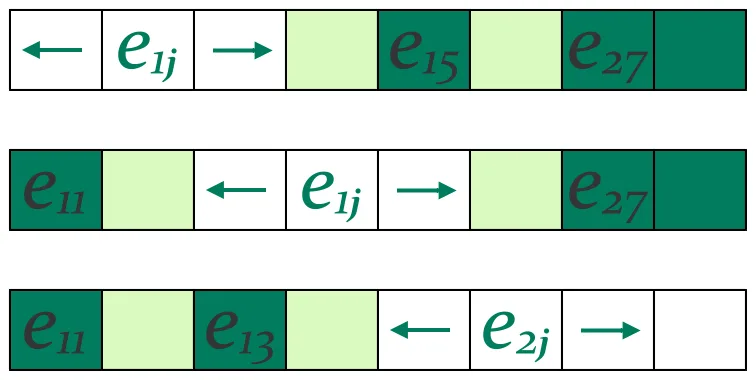
From the picture above, we see that,

$$\boxed{\begin{array}{l} 1 \,\leq\, e_{11} + e_{12} + e_{13} \,\leq\, 2 \\ 1 \,\leq\, e_{13} + e_{14} + e_{15} \,\leq\, 2 \\ 1 \,\leq\, e_{25} + e_{26} + e_{27} \,\leq\, 1. \end{array}}$$

As in Section 4c, the linear combination with coefficients of 1 counts how many blocks of a particular size appear. We used logic to narrow down the range where the blocks can appear. For certain, there is at least 1 block of that size in this range.

The upper bound is determined by how many other blocks of the same size appear in the range (i.e. number of overlaps among the ranges). For example, the upper bounds of $e_{11} + e_{12} + e_{13}$ and $e_{13} + e_{14} + e_{15}$ are 2, because we can place blocks of 1 cell on the 1st and 3rd columns (or on the 3rd and 5th columns) and the block of 2 cells afterward.

In summary, we follow this procedure for block order:

Consider the $I$-th row, where $I$ is a number between 1 and $m$.

1. If the row sequence has only one number, then do nothing.

2. If the row sequence has block sizes that do not repeat, then for each pair of consecutive blocks, create 2 inequalities such as those shown in the first approach. This strongly enforces the order.

3. If the row sequence has blocks sizes that repeat, then for each block, create 2 inequalities such as those shown in the second approach. This weakly enforces the order.

We arrive at the inequality $B_{2}\vec{x} \leq \vec{c}_{2}$. Note that we can change the strict inequalities in the first approach to inequalities with an equal sign if we add 1 to the smaller side. How large $B_{2}$ is depends on the row sequences and differs from one nonogram to another. The most rows that $B_{2}$ can have is $\sum_{i\,=\,1}^{m}\,2p_{i} = 2s$, when all row sequences have more than one number and have repeating block sizes.

f. Put it altogether

We created three sets of linear equations and two sets of linear inequalities. We can combine the linear equations into one equation: $A\vec{x} = \vec{b}$. Simply let,

$$A = \left[\begin{array}{c} A_{1} \\ \hline A_{2} \\ \hline A_{3} \end{array}\right] \in \mathbb{R}^{M_{1} \times N},\text{\hspace{0.5cm}} \vec{b} = \left[\begin{array}{c} \vec{b}_{1} \\ \hline \vec{b}_{2} \\ \hline \vec{b}_{3} \end{array}\right] \in \mathbb{R}^{M_{1}}.$$

The number of linear equality constraints is,

$$\boxed{\vphantom{\Bigl[\Bigr.}M_{1} = 1 + n + mn}.$$

Note that $M_{1}$ already exceeds the minimum number of measurements, $2s = \frac{m(n + 1)}{2}$, that is required for sparse recovery.

Similarly, we can combine the linear inequalities into one inequality: $B\vec{x} \leq \vec{c}$. Let,

$$B = \left[\begin{array}{c} B_{1} \\ \hline B_{2} \end{array}\right] \in \mathbb{R}^{M_{2} \times N},\text{\hspace{0.5cm}} \vec{c} = \left[\begin{array}{c} \vec{c}_{1} \\ \hline \vec{c}_{2} \end{array}\right] \in \mathbb{R}^{M_{2}}.$$

The number of linear inequality constraints depends on the nonogram. However, we have a bound for $M_{2}$:

$$\boxed{\vphantom{\Bigl[\Bigr.}mn \leq M_{2} \leq mn + 2s}.$$

Notes

Allow me to explain why, in compressive sensing, we want to minimize the 1-norm of the solution vector:

$$||\vec{x}||_{1} \,=\, |x_{1}| \,+\, |x_{2}| \,+\, \cdots \,+\, |x_{N}|.$$

After all, isn't the 2-norm of a vector (Euclidean distance)

$$||\vec{x}||_{2} \,=\, \sqrt{\vphantom{\bigl[\bigr.}x_{1}^{2} \,+\, x_{2}^{2} \,+\, \cdots \,+\, x_{N}^{2}}$$

more commonly used?

The solution $\vec{x}$ lives in an $N$-dimensional space, which may be hard to imagine. For now, just imagine a 2D space. Over there, the linear constraints $A\vec{x} = \vec{b}$ and $B\vec{x} \leq \vec{c}$ become a line.

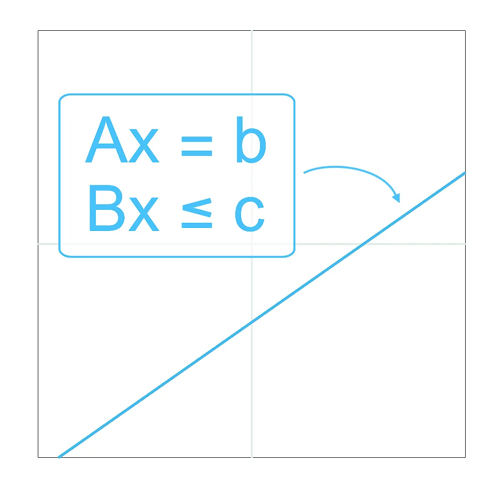
We want a solution $\vec{x}$ that lies on the line (meets the constraints) and has the smallest size (when measured in 1-norm or 2-norm). Define the $l^{1}$-ball of radius $R$ to be the set of all vectors whose 1-norm equals $R$, and similarly define the $l^{2}$-ball.

In 2D, the $l^{1}$-ball always takes the shape of a square diamond, and the $l^{2}$-ball, a circle. First, consider drawing $l^{1}$-balls that get smaller and smaller in size:

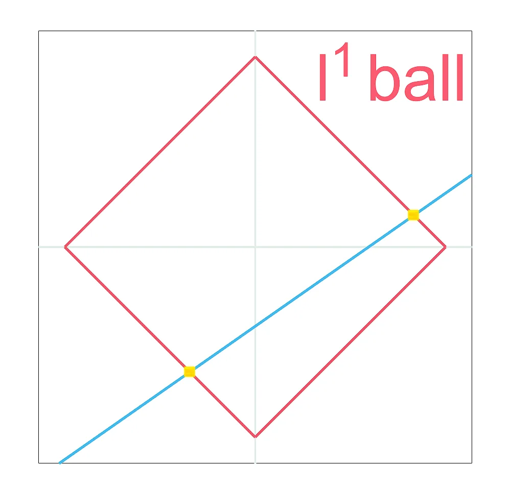
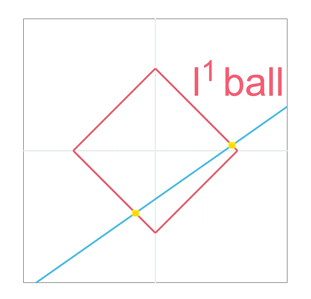
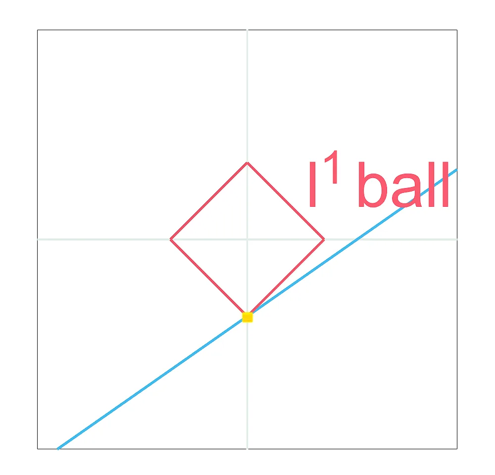
An intersection between the ball and the line represents a solution $\vec{x}$. The solution that we want occurs when the ball is just small enough, so that, if it becomes any smaller, it would not intersect the line anywhere.

Notice that the minimizer $\vec{x}$ lies on an axis. We know that points on an axis have one coordinate that is equal to 0. Similarly, the minimizer (a vector) has one entry that is 0. This is in 2D. In $N$ dimensions, the minimizer will likely have many entries that are 0, resulting in a vector that is sparse.

Now, consider drawing $l^{2}$-balls that get smaller and smaller in size:

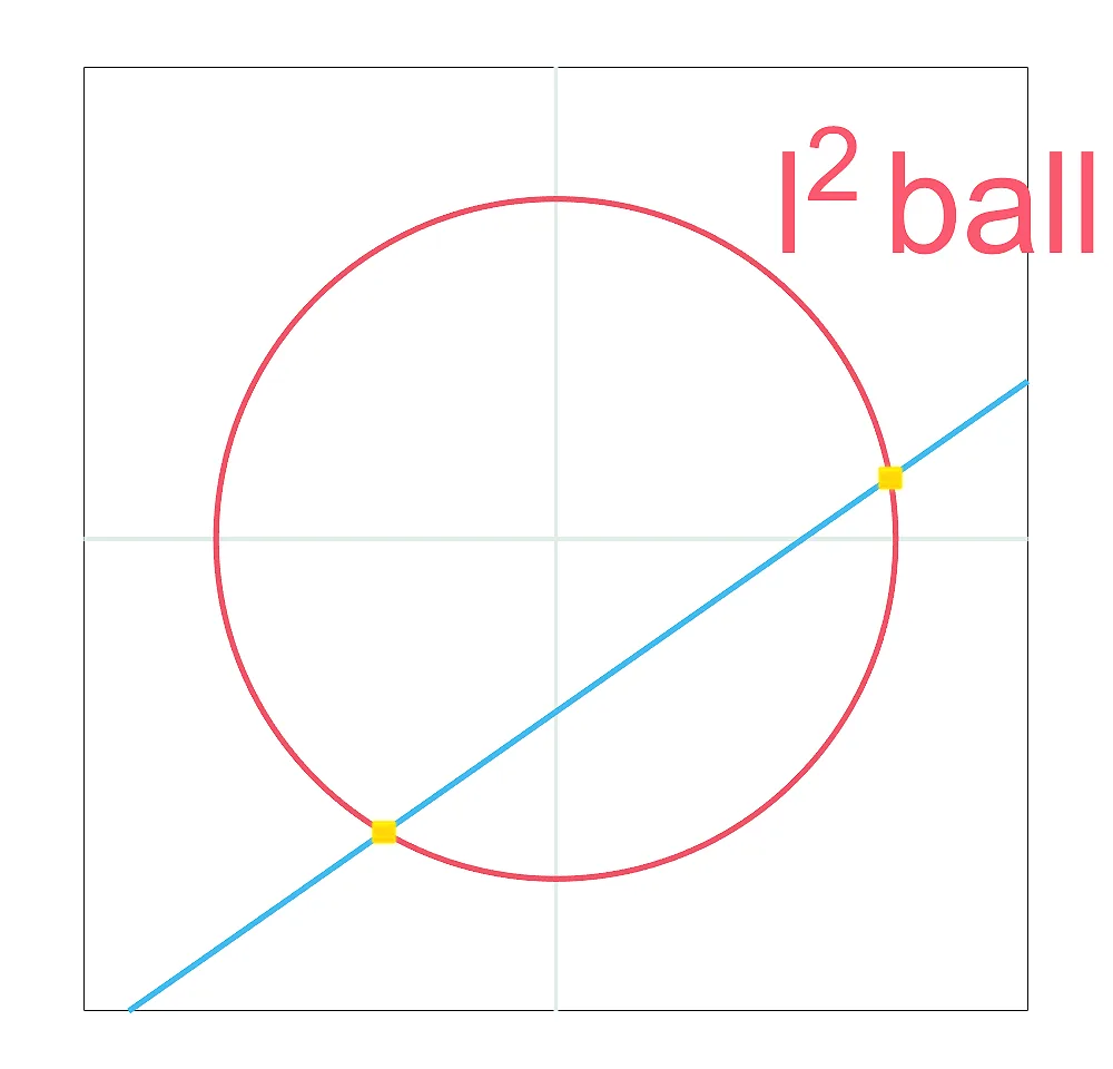
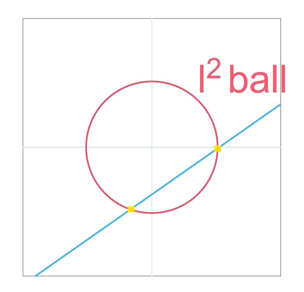
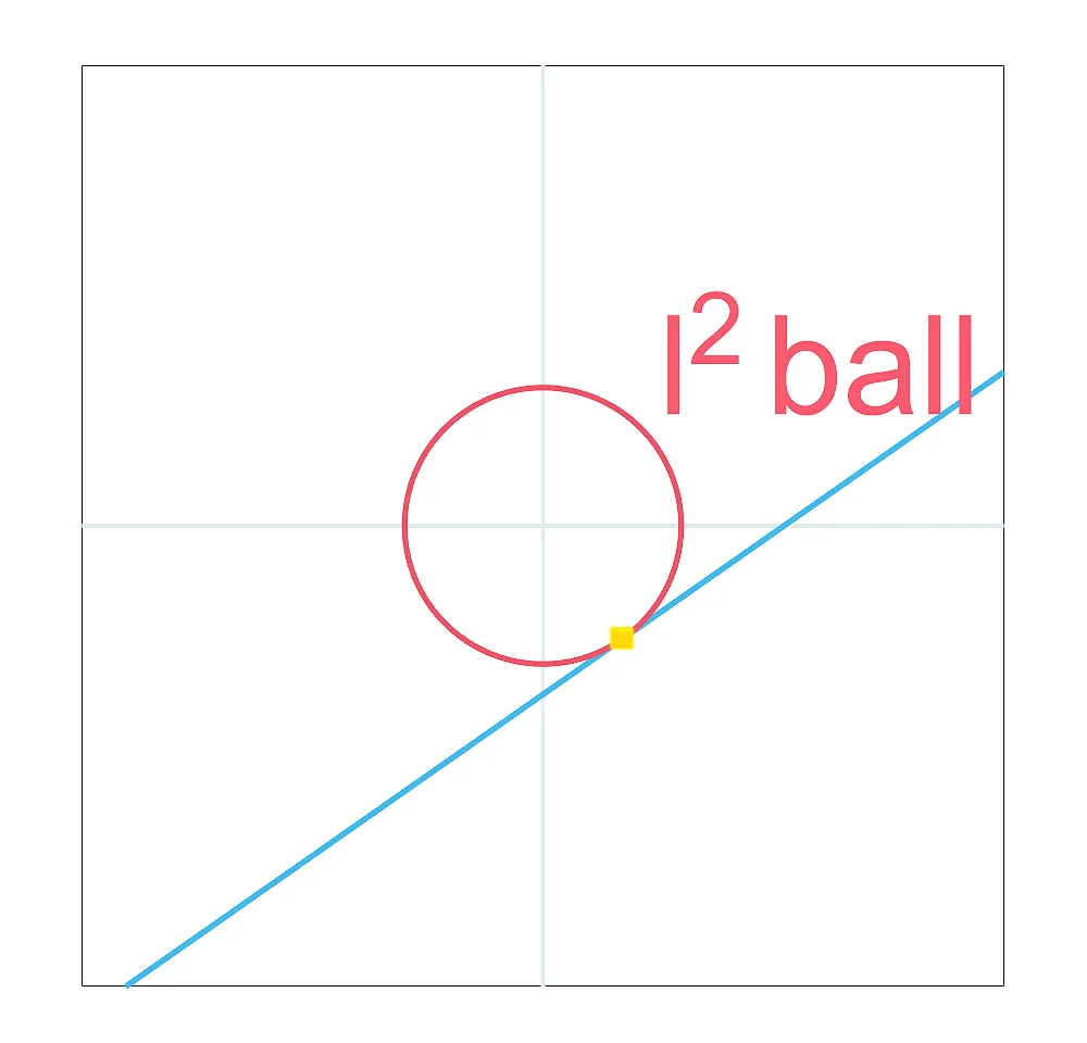
This time, the minimizer does not land on an axis. Its two entries are both nonzero. By the same token, in $N$ dimensions, the minimizer will likely have many nonzero entries, resulting in a vector that is not sparse.