Solving Nonograms with Compressive Sensing: Part 2

3. Introducing compressive sensing

Today, we will consider how to turn the solution of a nonogram into a sparse vector. But first, let me take a detour and illustrate an approach that Oscar and I initially had considered and comment on its strengths and weaknesses in solving the puzzle.

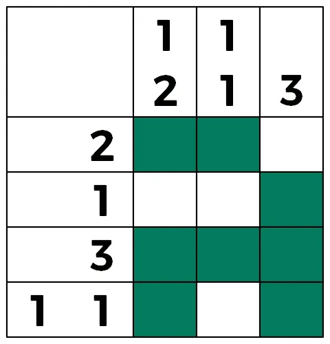
Throughout our discussion, we will consider the stylish lambda example:

a. Initial attempt

We can indicate whether a cell needs to be empty or shaded with a binary number. Since a nonogram involves an $m \times n$ grid, it's natural to imagine the solution as a matrix $X \in \{0,\,1\}^{m \times n}$. By listing the entries in single file, we can also think of the solution as a vector $\vec{x} \in \{0,\,1\}^{N}$, with

$$N = mn.$$

(The notations $\{0,\,1\}^{m \times n}$ and $\{0,\,1\}^{N}$ refer to the set of matrices with binary entries and the set of vectors with binary entries.)

The $(i,\,j)$-th cell uniquely corresponds to $x_{k}$, the $k$-th entry in the vector $\vec{x}$. We let $k = (i - 1)n + j$, for example. Then, assign $x_{k} = 0$ if the cell should be empty, and $x_{k} = 1$ if shaded.

The solution to the stylish lambda is given by a vector $\vec{x} \in \{0,\,1\}^{12}$, where

$$\vec{x} = \bigl[ \,\,1\,\, \,\,1\,\, \,\,0\,\, \,|\, \,\,0\,\, \,\,0\,\, \,\,1\,\, \,|\, \,\,1\,\, \,\,1\,\, \,\,1\,\, \,|\, \,\,1\,\, \,\,0\,\, \,\,1\,\, \bigr]^{T}.$$

If we assume that a nonogram had been created randomly, then Lemma 2.1 says that half of the cells would be shaded. In other words, we can expect the sparsity level $s$ (the number of nonzero entries) of the solution $\vec{x}$ to be,

$$\displaystyle\mathbb{E}(s) = \frac{mn}{2}.$$

Compressive sensing asks us to provide at least $2s = mn$ measurements for sparse recovery of $\vec{x}$, with an extra multiplicative factor of $\ln\bigl(\frac{N}{s}\bigr) = \ln(2)$ for stability. Rather fortunately, this factor is constant on average and independent of the puzzle size.

The problem is, it is not clear how to group cells to faithfully represent the row and column sequences. Consider the stylish lambda. The first row sequence $(2)$ means we must shade a block of 2 cells. How do we express the idea of "a group of cells" when each entry of $\vec{x}$ stands for a single cell?

One way is to enumerate all possibilities, e.g. we require that

$$x_{1}x_{2} = 1 \,\,\,\text{or}\,\,\, x_{2}x_{3} = 1,$$

but this creates additional problems. These constraints are nonlinear, the degrees of these constraints equal the block size (i.e. for larger blocks, the nonlinearity is more severe), and the solver that we use may not handle a logical operator such as "or."

Furthermore, for sequences like $(1,\,1)$ and $(1,\,2)$ with more than one number, we must also specify that there exist empty cells between any two consecutive blocks of cells. We do not know upfront how many empty cells there are, however. Again, we could consider all possibilities, but Theorem 2.3 tells us that doing this is very unwise.

Probably the best that we can do is to impose the row and column sequences weakly. For example, we require that the row sums and the column sums are satisfied. These, we can easily do with $(m + n)$ linear equations. However, the number of equations is nowhere close to $2s = mn$ that is needed for sparse recovery.

b. Our solution

The main problems of representing the solution as a vector $\vec{x}$ as described above are that (1) it is hard to group cells and (2) to indicate that, in certain places, there needs to be empty cells.

We can come to a new insight by considering the stylish lambda and one of its rows, which has $n = 3$ cells:

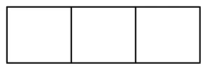
There are $\frac{n(n + 1)}{2} = 6$ possible ways to shade a block of cells in this row. Mainly,

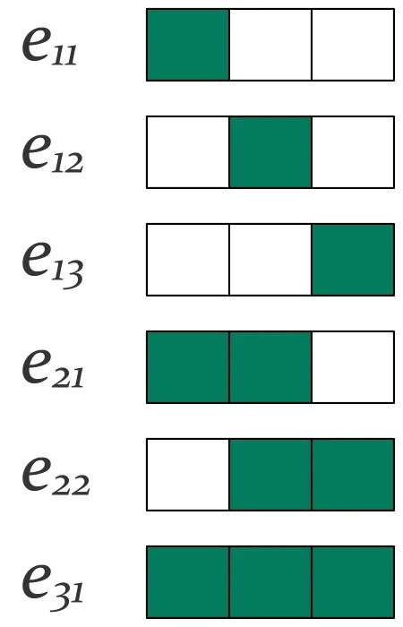
As shown above, we label these six objects by

$$e_{kj},$$

where $k$ is the size of the block of shaded cells, and $j$ is the starting column position of the block. (We listed the indices $k$ and $j$ in an "odd" manner, because it's easier to say what $e_{kj}$ does in words. For example, we would say that $e_{21}$ means "shade a block of 2 cells starting at the first column.")

Despite the conflict in terminologies, we call these six objects the (row) basis vectors, because we can write every row sequence as a unique sum of these basis vectors. For the stylish lambda,

we can represent rows 1 and 4 as,

$= \underbrace{e_{11}}_{=\,0} + \underbrace{e_{12}}_{=\,0} + \underbrace{e_{13}}_{=\,0} + \underbrace{e_{21}}_{=\,1} + \underbrace{e_{22}}_{=\,0} + \underbrace{e_{31}}_{=\,0}$

$= \underbrace{e_{11}}_{=\,1} + \underbrace{e_{12}}_{=\,0} + \underbrace{e_{13}}_{=\,1} + \underbrace{e_{21}}_{=\,0} + \underbrace{e_{22}}_{=\,0} + \underbrace{e_{31}}_{=\,0}$.

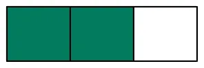
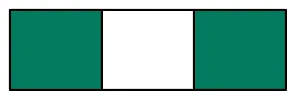
We did not write $e_{11} + e_{12} + e_{13} + e_{21} + e_{22} + e_{31} = 1 + 1 + 0 + 0 + 0 + 0$ for row 1, because this violates the nonogram rule that two consecutive blocks are separated by empty cell(s). As long as we can enforce this rule, we would get a unique sum.

Since we can create these basis vectors for each row, let us insert an index $i$ to denote the row position of a basis vector. Hence, every basis vector has the name

$$\boxed{e_{ikj},\,\,\text{where}\,\,\left\{\begin{array}{l} i = 1,\,\cdots,\,m \\ k = 1,\,\cdots,\,n \\ j = 1,\,\cdots,\,n - k + 1. \end{array}\right.}$$

Sometimes, we will arrive at a result that holds true for any row. In such cases, we will suppress the index $i$ for simplicity. Also, we will use $e_{ikj}$ to mean the name of the basis vector as well as the binary variable that indicates whether to shade a block of $k$ cells starting at the $(i,\,j)$-th position. It will be obvious from the context to which we refer.

Let us store $e_{ikj}$ as entries of a vector $\vec{x} \in \{0,\,1\}^{N}$. Note that,

$$\displaystyle\boxed{N = \frac{mn(n + 1)}{2}}.$$

The solution to the stylish lambda is given by $\vec{x} \in \{0,\,1\}^{24}$, where

$$\begin{aligned} \vec{x} &= \bigl[ \,\,e_{111}\,\, \,\,e_{112}\,\, \,\,e_{113}\,\, \,\,e_{121}\,\, \,\,e_{122}\,\, \,\,e_{131}\,\, \,\cdots\, \,\,e_{411}\,\, \,\,e_{412}\,\, \,\,e_{413}\,\, \,\,e_{421}\,\, \,\,e_{422}\,\, \,\,e_{431}\,\, \bigr]^{T} \\ &= \bigl[\,\,0\,\, \,\,0\,\, \,\,0\,\, \,\,1\,\, \,\,0\,\, \,\,0\,\, \,|\, \,\,0\,\, \,\,0\,\, \,\,1\,\, \,\,0\,\, \,\,0\,\, \,\,0\,\, \,|\, \,\,0\,\, \,\,0\,\, \,\,0\,\, \,\,0\,\, \,\,0\,\, \,\,1\,\, \,|\, \,\,1\,\, \,\,0\,\, \,\,1\,\, \,\,0\,\, \,\,0\,\, \,\,0\,\, \bigr]^{T}. \end{aligned}$$

We call the manner in which we have listed the variables $e_{ikj}$ in the solution vector $\vec{x}$ as the natural order of the basis vectors.

Our new approach allows the solution vector $\vec{x} \in \{0,\,1\}^{N}$ to be sparse. For any row sequence, we will likely need only a few basis vectors to represent the sequence. For the stylish lambda, we used 5 basis vectors out of the possible 24. This is because 5 numbers appear in the row sequences.

Had a nonogram been created randomly, Lemma 2.1 says that, on average, each row has $\frac{n + 1}{4}$ blocks of shaded cells. This means, we can recreate each row with $\frac{n + 1}{4}$ basis vectors. Hence, we expect the sparsity level $s$ to be,

$$\displaystyle\boxed{\mathbb{E}(s) = \frac{m(n + 1)}{4}}.$$

This is nearly half of that from our initial approach, meaning we could make fewer measurements and reconstruct the solution. The logarithmic factor for stability is now $\ln(2n)$, but this increases very slowly if the column size increases.

Furthermore, there is a huge prize: We can easily indicate a block of shaded cells now, thanks to the very construction of the basis vectors. Each number in a row sequence indicates a block of shaded cells, which corresponds to a particular basis vector.

By now, you may have noticed that the basis vectors lie along just one direction. Next time, I will detail how to build constraints from the nonogram, including those that say empty cells must exist between any two consecutive blocks. We will see that we can easily extract information from the row sequences but not from the column sequences.

Of course, we can also create basis vectors for a column so that we make a better use of the column sequences. At the end of the series, I will show the benefits of doing so.

Notes

We discussed the sparsity level in terms of its expected value. For analysis, it is more convenient and meaningful to consider the expectation, which (as we saw above) is a function "directly" of the size of the puzzle. However, we do know the exact value.

In the first approach, the sparsity level is equal to,

$$\displaystyle s = \sum_{i\,=\,1}^{m}\,r_{i},$$

the sum of all the row sums. It is also equal to the sum of all the column sums.

In the second approach, it is,

$$\displaystyle s = \sum_{i\,=\,1}^{m}\,p_{i},$$

the total number of blocks of shaded cells (row-wise), or equivalently, how many numbers appear in the row sequences.