In numerical linear algebra, we create ways for a computer to solve a linear system of equations Ax=b. In doing so, we analyze how efficiently and accurately we can find the solution x.
Perturbation theory concerns how much error we incur in the solution x when we perturb (spoil) the data A and b. A classic statement tells us that the amount of error depends on the condition number of the matrix A.
I will define and prove the statement, and help you understand it by "hearing" it.
1. Problem statement
Let's consider the equation,
Axtrue=b,
where A∈Rn×n is nonsingular and b=0 (otherwise, we get the trivial case xtrue=0). Note that xtrue denotes the true solution. It's what we hope to get.
Suppose, instead, we solve the perturbed system,
(A+δA)x=b+δb.
We seek to find a bound on the error x−xtrue. We expect the error to be small when δA and δb are small changes.
Given an induced matrix norm∣∣⋅∣∣, we can define the condition number of A:
κ(A):=∣∣A∣∣⋅∣∣A−1∣∣.
Note that we always have κ(A)≥1. You can check why, along with the definition and properties of an induced matrix norm, in Notes.
We will show that, under a mild assumption κ(A)⋅∣∣A∣∣∣∣δA∣∣<1,
The RHS is a product of terms, so we can conclude two things. (1) If κ(A) is a small number, then small relative errors in A and b will result in a small relative error in the solution xtrue. (2) If κ(A) is a large number, however, we may get a large relative error in xtrue even when the relative errors in A and b are small.
We see that the condition number influences how much change occurs in the output when we change the input of a system. As a result, we say that the matrix A is well-conditioned if κ(A) is small, and ill-conditioned if κ(A) is large.
2. Mathematical proof
a. Step 1
For any matrix X∈Rn×n with ∣∣X∣∣<1, the following statements hold:
(i) I−X is nonsingular, and its inverse is given by
(I−X)−1=i=0∑∞Xi=I+X+X2+⋯.
(ii) ∣∣(I−X)−1∣∣≤1−∣∣X∣∣1.
To prove (i), we check that (I−X)(I−X)−1=I and (I−X)−1(I−X)=I. We just need to check one of them because, in finite dimensions, injectivity and surjectivity occur together.
Note, to be rigorous, we would first show that the infinite series ∑i=0∞Xi converges. The sequence of finite sums, {∑i=0kXi}k=0∞, is a Cauchy sequence in the norm ∣∣⋅∣∣. Since Rn×n is a Banach space, i.e. complete, the sequence converges.
Let's prove (ii). By triangle inequality and the properties of an induced matrix norm,
Next, we use the infinite geometric sum formula: For any real number r∈(−1,1),
i=0∑∞ri=1−r1.
Since ∣∣X∣∣∈[0,1), we conclude that,
∣∣(I−X)−1∣∣≤1−∣∣X∣∣1.
■
b. Step 2
Recall that A is nonsingular. Assume further that,
κ(A)⋅∣∣A∣∣∣∣δA∣∣<1.
Then, A+δA is also nonsingular.
Since A is nonsingular, we can write A+δA as a product of two terms:
A+δA=A(I+A−1δA).
Hence, A+δA is nonsingular, if and only if, I+A−1δA is nonsingular. Let's show that the latter is true by applying (i) from Step 1.
We find that,
∣∣A−1δA∣∣≤∣∣A−1∣∣⋅∣∣δA∣∣=κ(A)∣∣A∣∣∣∣δA∣∣<1.
Hence, I+A−1δA is nonsingular.
■
Before we move on, let's read the statement in Step 2 again. It tells us that, if a matrix is nonsingular, then there are infinitely many matrices nearby that are nonsingular, too. (And infinitely many around them, and so on.) This supports the fact that there are far more nonsingular matrices than singular ones. Isn't that a marvel?
We can represent an audio as a vector xtrue∈Rn of frequencies. The provided audio file, williams.wav, lends to n=189930. At a sampling rate of 44100 Hz, the audio is 4.3068 seconds long.
For computational efficiency, we will write xtrue as a matrix Xtrue∈R10×18993, by storing the first 10 entries of xtrue as the first column of Xtrue, the next 10 entries as the second, and so on.
Next, we apply a nonsingular matrix A∈R10×10 to Xtrue to get the encrypted audio B∈R10×18993. We can always vectorize B into b∈R189930 by reversing the storage process described above.
From now on, we assume that we only have A and B. We seek to decrypt the audio, i.e. solve the equation AXtrue=B, when there are perturbations in the matrix A and/or in the input B:
(A+δA)X=(B+δB).
a. Generating matrices
To generate a well-conditioned A, we find the QR factorization of a random 10×10 matrix and set A=Q. We know that the 2-norm of an orthogonal matrix is always 1. Hence,
κ2(Q)=∣∣Q∣∣2⋅∣∣QT∣∣2=1.
For an ill-conditioned A, we use the Hilbert matrix H:
Then, κ2(H)≈1.6025×10¹³. Note that both Q and H are nonsingular.
b. Generating perturbations
The entries of perturbations δA and δB are randomly generated from a scaled normal distribution. For convenience, we will assume that A+δA is (most likely) nonsingular because δA is randomly chosen.
We are more interested in ensuring that the values of ∣∣δA∣∣2 and ∣∣δb∣∣2 stay about the same each time we run the program.
c. Simulations
We can run perturbation_theory.m under 6 different cases:
The table lists the input parameters for each case.
First, let's consider what happens when A is well-conditioned.
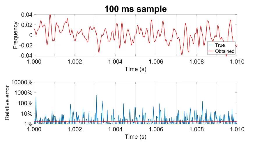
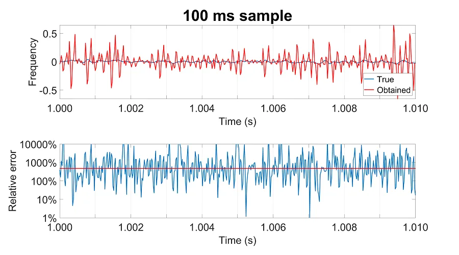
Fig 1a. Well-conditioned matrix, perturbation to A only.
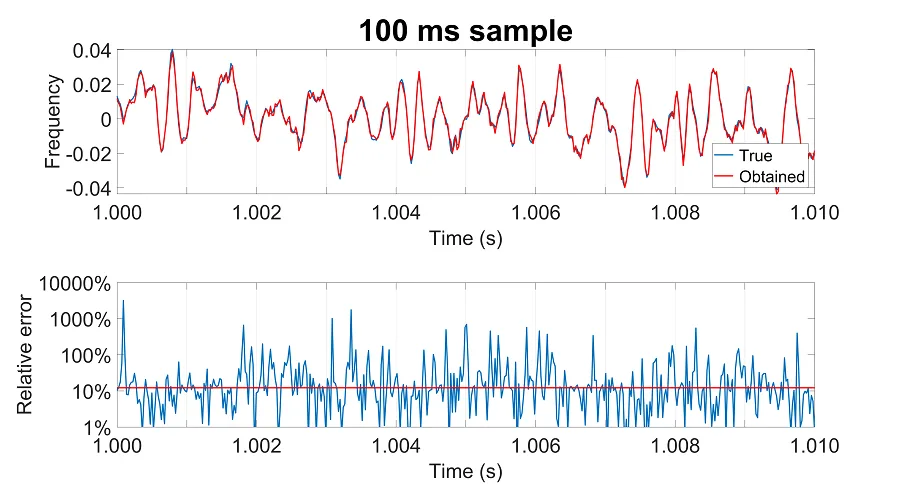
Fig 1b. Well-conditioned matrix, perturbation to B only.
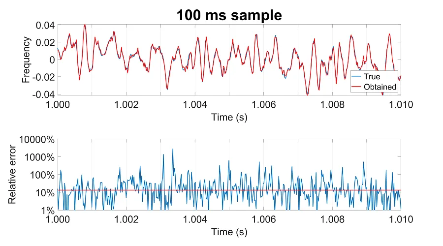
Fig 1c. Well-conditioned matrix, perturbation to both A and B.
These plots show that the obtained solution x matches the true solution xtrue well. The fidelity of the obtained audios remains largely pristine. We do hear some added noise. In the 100 ms sample, the relative error stays around 2% (median) when we perturb only the matrix A. When we perturb the encrypted audio B, the relative error jumps to about 10%.
Next, let's consider what happens when A is ill-conditioned.
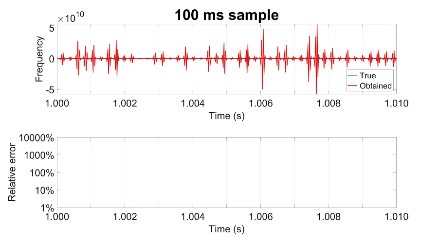
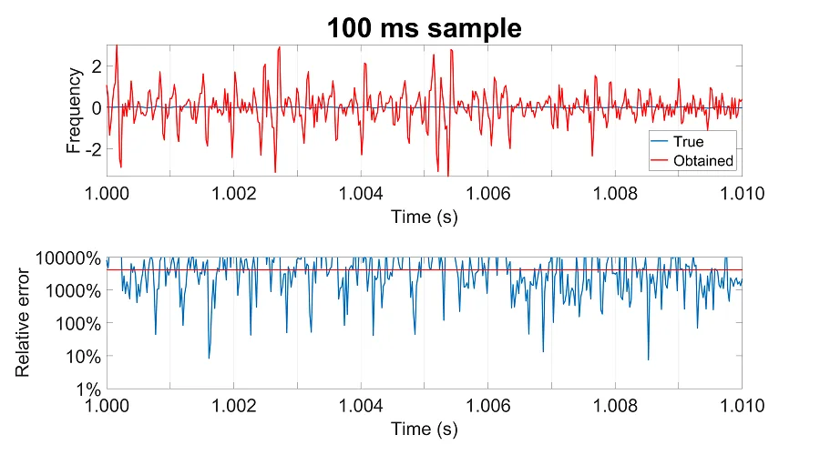
Fig 2a. Ill-conditioned matrix, perturbation to A only.
Fig 2b. Ill-conditioned matrix, perturbation to B only.
Fig 2c. Ill-conditioned matrix, perturbation to both A and B.
This time, the obtained solution hardly matches the true solution. You can hear much more noise in the obtained audios, and listening to them becomes almost unbearable. The relative error is orders of magnitude larger. It's interesting how perturbing B only results in a completely garbled audio, but perturbing A in addition reconstructs some of the original audio. Two wrongs do make a right, it seems.
We can also check that our matrices satisfy the statement that we painstakingly proved. I will leave writing the extra code to you.
Notes
Given a vector norm ∣∣⋅∣∣ for the vector space Rn, we can always create a matrix norm ∣∣⋅∣∣ for the vector space Rn×n. As a result, we call this an "induced" matrix norm. For simplicity, I use the double bar notation for both types of norms. It is clear from context whether we are looking at the vector norm or the induced matrix norm.
The induced matrix norm of A∈Rn×n is defined as,
∣∣A∣∣:=x=0max∣∣x∣∣∣∣Ax∣∣=∣∣x∣∣=1max∣∣Ax∣∣.
Hence, the induced matrix norm measures how far out we can map a vector relative to its original size. We can also generalize the definition to rectangular matrices.
Because of its definition, the induced matrix norm satisfies these useful properties:
(i) For any A∈Rn×n and x∈Rn,
∣∣Ax∣∣≤∣∣A∣∣⋅∣∣x∣∣.
(ii) For any A,B∈Rn×n,
∣∣AB∣∣≤∣∣A∣∣⋅∣∣B∣∣.
In particular, property (ii) implies that the condition number of a nonsingular matrix is always at least 1.
AA−1=I⇒∣∣AA−1∣∣=1⇒∣∣A∣∣⋅∣∣A−1∣∣≥1.
You can find the code and audio files in their entirety here: Download from GitHub